2. Theoretical Background
ABCluster is designed as a black-box program: a global optimization can be performed without a detailed knowledge of the underlying theory. Nevertheless, a working understanding of the potential energy surface, the search algorithm, and the choice of energy method will make the calculations more reliable and the results easier to interpret. This chapter summarizes the essential ideas used in ABCluster.
The following topics are covered:
why local optimization is insufficient, and what global optimization actually seeks;
how conformation search is unified with cluster global optimization;
how to choose an energy evaluation method under the constraint of computational cost;
how the artificial bee colony (ABC) algorithm works, and how to set its parameters;
automatic atom typing for CHARMM-type calculations;
many-body energy decomposition analysis (MB-EDA) for interpreting cluster stability.
2.1. Global Optimization
Tip
For a broader survey of global optimization of chemical clusters, the following review is strongly recommended:
Zhang, J.; Glezakou, V.-A. Global Optimization of Chemical Cluster Structures: Methods, Applications, and Challenges. Int. J. Quantum Chem. 2021, 121, e26553.
2.1.1. The Potential Energy Surface
A cluster is an aggregate of structural units (atoms, ions, rigid molecules, or flexible molecules). Different packing arrangements of these units generally give different energies. The energy difference between two isomers can be smaller than 1 kcal mol-1, yet their geometries and chemical properties may differ substantially.
The set of all nuclear arrangements, together with the energy of each arrangement, defines the potential energy surface (PES). Two types of stationary points on the PES are of particular importance:
A local minimum (LM) is a structure at which the energy gradient vanishes and all vibrational frequencies are real. Chemically, LMs correspond to isomers (or conformers). Neighbouring LMs are separated by energy barriers.
The global minimum (GM) is the LM of lowest energy on the PES (for a given composition, charge, and spin state). It is the thermodynamically most stable isomer at zero temperature, neglecting entropy.
2.1.2. Local versus Global Optimization
If a cluster is constructed by randomly packing its structural units, a local optimization (for example OPT in Gaussian, or integrator = cg in GROMACS) will only relax the structure into the nearest LM. Because the PES of a cluster typically contains a large number of LMs, that nearest basin is often high in energy and chemically unrepresentative. Local optimization cannot cross barriers, so it cannot, by itself, locate the GM.
Global optimization is an algorithm that searches for the GM by combining local relaxation with operators that allow the search to leave LM traps. The operators determine the character of the algorithm. Common choices include basin hopping, genetic algorithms, and the artificial bee colony (ABC) algorithm. ABC requires only three parameters or fewer, and is therefore easy to learn and to control. It is the core search engine of ABCluster.
2.1.3. The Putative Nature of the Global Minimum
An LM can be identified rigorously by a vanishing gradient (and a positive-definite Hessian). There is no equally robust numerical test for a GM. Any GM reported by ABCluster, or by any other global optimization program, should therefore be regarded as a putative GM.
In practice, the following checks are recommended:
Inspect the putative GM with chemical intuition: is a more stable packing conceivable?
Repeat the search with different random seeds, population sizes, or generation numbers, and compare the lowest-energy structures.
For small systems, increase the computational budget until the same GM is recovered in independent runs.
Tip
The practical capability of global optimization depends strongly on system size:
For small clusters (number of structural units \(< 25\)), modern algorithms can usually locate the true GM at an acceptable cost. For systems such as \(\mathrm{Cu}_{16}\) or \(\left(\mathrm{NH}_3\right)_{15}\), a serious attempt to find the true GM is warranted.
For large clusters, a mathematically guaranteed GM cannot be claimed. A structure of very low energy can nevertheless be obtained, and in many applications that structure is sufficient for subsequent theoretical analysis.
2.1.4. The Value of Local Minima
A global optimization with ABCluster produces not only the putative GM, but also a large set of LMs. These structures map out the low-energy region of the PES. Experimental observables are often determined by an ensemble of low-lying isomers rather than by the GM alone. The LMs should therefore be examined together with the GM.
Tip
An illustration is the global optimization of \(\mathrm{Au}_8\) supported on graphene oxide (GO), reported here. In the GM and in one LM, some gold atoms form covalent bonds with oxygen atoms of GO. In other LMs, no such bonds are formed, and the most stable member of that family resembles the gas-phase GM of \(\mathrm{Au}_8\). The PES therefore falls into two families: “GO-corrupted” and “GO-uncorrupted” clusters. In the latter family, GO has little effect on the stability order of the \(\mathrm{Au}_8\) isomers.
2.2. Conformation Search
A flexible molecule possesses flexible degrees of freedom (DOFs), typically rotatable single bonds and deformable rings. As on a cluster PES, these DOFs generate many conformers separated by barriers. In organic and medicinal chemistry, conformation often controls reactivity and binding.
From the viewpoint of optimization, conformation search is the same problem as cluster global optimization: both are global searches on a PES. The only difference is the definition of the search variables. Since ABCluster 3.0, conformation search and cluster global optimization have been unified and can be performed in a single calculation:
conformation search is global optimization of a cluster that contains one flexible molecule;
cluster global optimization is a search over both the packing of structural units and the internal deformation of those units.
Flexibility can be assigned independently for each structural unit. Selected bonds or rings may be frozen. If every DOF of a unit is frozen, that unit is treated as a rigid body.
Tip
A typical example is a xylitol cluster. The conformation of the xylitol carbon chain determines the spatial arrangement of the hydroxyl groups, and therefore the hydrogen-bonding network of the cluster. A reliable GM requires simultaneous sampling of intramolecular flexibility and intermolecular packing.
Tip
When a ligand is placed in the active pocket of a protein, the ligand conformation and its rigid-body position and orientation must be optimized together. In some cases the flexibility of pocket residues should also be included.
2.3. Energy Evaluation
2.3.1. Two Competing Requirements
Global optimization locates structures of low energy. The energy method must therefore satisfy two, often conflicting, requirements:
Reliability. The ranking of isomers must be chemically correct. The choice among DFT functionals, semi-empirical methods, and force fields should be based on computational experience, literature benchmarks, or a short calibration on representative structures before a production search.
Cost. Accuracy is expensive. The following table gives a rough order of magnitude for the cost of one local optimization, taking a typical force-field evaluation as unity:
Method |
Relative cost |
|---|---|
Force fields |
1 |
Semi-empirical methods |
1,000 |
ab initio methods (gas phase) |
10,000–100,000 |
ab initio methods (periodic systems) |
300,000–1,000,000 |
A reliable global optimization commonly requires 500 to 10,000 or more local optimizations. A direct search at a high ab initio level is therefore rarely feasible. A compromise between reliability and cost is unavoidable.
2.3.2. A Hierarchical Protocol
A useful rule of thumb is: explore first with a cheaper but still reasonable method, then refine the surviving structures with higher-level calculations. A typical hierarchy is:
global search with a force field or a fast semi-empirical method, collecting a large pool of LMs;
reoptimization of that pool at a better semi-empirical or DFT level, discarding high-energy isomers;
tighter DFT optimization of the remaining low-energy structures;
single-point energy evaluation of a shortlist with a high-level wave-function method, if needed.
Tip
In atmospheric chemistry, molecular clusters must be ranked with an accuracy that force fields alone cannot guarantee. This paper describes a systematic protocol of this kind:
Global optimization with ABCluster at the CHARMM force-field level, yielding 10,000 LMs.
Reoptimization of the 10,000 LMs at the GFN-xTB level. After high-energy structures are discarded, about 1,000 remain.
Optimization of the 1,000 clusters at the \(\omega\)B97X-D/6-31++G(d,p) level with loose convergence criteria, followed by tight reoptimization of selected low-energy isomers.
DLPNO-CCSD(T)/aug-cc-pVTZ single-point energies for the 10 lowest-lying clusters.
The same idea can be adapted to other chemical systems by changing the methods at each stage.
2.3.3. When the CHARMM Force Field Is Appropriate
Clusters composed of ordinary organic molecules and closed-shell inorganic ions are often described adequately by the CHARMM force field. In that situation rigidmol (or the internal CHARMM engine of geom) is a suitable first tool, and an expensive quantum-chemical search from the outset is unnecessary. The low-energy candidates must still be reoptimized and ranked with ab initio methods before chemical conclusions are drawn.
2.3.4. When a Quantum-Chemical Method Is Required
Clusters whose electronic structure is delocalized, open-shell, or otherwise poorly represented by pairwise classical potentials should be treated quantum-chemically from the beginning. “Quantum-chemical” here includes both semi-empirical methods (for example GFN2-xTB) and ab initio methods (for example DFT). Typical cases are:
Atomic clusters, for example \(\mathrm{Au}_{20}\) and \(\mathrm{B}_8\mathrm{N}_8\).
Inorganic clusters with metal–ligand bonding, for example \(\mathrm{Co}_6\mathrm{Te}_8(\mathrm{PEt}_3)_6\).
Clusters with extra or missing electrons, or with unusual spin multiplicities, for example \((\mathrm{H}_2\mathrm{O})_{10}^{-}\). The phrase “extra or missing electrons” must be interpreted chemically: a sodium cation is a closed-shell species and can be described by CHARMM, whereas a sodium atom requires a quantum-chemical treatment.
Periodic systems, such as surface-supported clusters. ABCluster should then be coupled to a periodic code such as CP2K or VASP.
2.3.5. Caution with Model Potentials
The component atom provides several model potentials developed for specific physical purposes. They are not systematic approximations to ab initio theory, and they are used more often in physics than in chemistry. When they are applied to a chemical problem, the user must know the range of validity of the potential and interpret the GM with care.
Attention
Gupta-type potentials are popular for metallic clusters. They are usually parametrized against condensed-phase properties and can be a poor choice for small clusters. For \(\mathrm{Au}_{20}\), DFT yields a tetrahedral GM consistent with experiment, whereas a Gupta potential yields an irregular polyhedral GM. The latter is chemically misleading. For a large cluster such as \(\mathrm{Au}_{80}\), where only a reasonable initial guess is required, the same Gupta potential can still be useful.
2.4. The Artificial Bee Colony Algorithm
Tip
The original descriptions of ABC as implemented in ABCluster are:
Zhang, J.; Dolg, M. ABCluster: The Artificial Bee Colony Algorithm for Cluster Global Optimization. Phys. Chem. Chem. Phys. 2015, 17, 24173-24181.
Zhang, J.; Dolg, M. Global Optimization of Clusters of Rigid Molecules Using the Artificial Bee Colony Algorithm. Phys. Chem. Chem. Phys. 2016, 18, 3003-3010.
2.4.1. Idea of the Algorithm
The ABC algorithm was proposed by Karaboga in 2005. It mimics the foraging behaviour of a honey-bee colony. Three types of bee are distinguished:
Employed bees (EM) explore the neighbourhood of a food source that is already known;
Onlooker bees (OL) choose among the known sources according to their quality and search further in promising regions;
Scout bees (SC) abandon exhausted sources and start a search in a completely new region.
After repeated cycles of these three operations, the colony concentrates on the best nectar. In ABCluster the “food source” is a cluster structure and the “nectar quality” is the energy (lower is better). The three bee types become three operators that generate new candidate structures from the current population.
The search balances exploitation (EM and OL operators refine known low-energy basins) and exploration (the SC operator injects new, unrelated structures). That balance is the reason ABC performs well on the highly multimodal PES of clusters.
2.4.2. Flowchart
A global optimization in ABCluster proceeds as follows:
Set the generation counter \(g = 0\).
Generate a population of \(SN\) cluster structures at random.
In generation \(g\), apply the EM, OL, and SC operators in turn. Each operator produces new candidate clusters.
Locally optimize every new candidate with the chosen energy method.
Update the population (a better candidate replaces a worse member).
If \(g \ge g_{\mathrm{max}}\), stop; otherwise set \(g \leftarrow g+1\) and return to step 3.
2.4.3. Parameters
A typical ABC search is controlled by three parameters. An estimate of the cluster size is sometimes also required:
\(SN\): population size. A larger population covers more of the PES, at a proportional increase in cost.
\(g_{\mathrm{max}}\): maximum number of generations. This is the principal budget of the search.
\(g_{\mathrm{limit}}\): scout limit. If a population member has not improved for \(g_{\mathrm{limit}}\) generations, it is abandoned and replaced by a new random structure. This is the main diversity-preserving mechanism.
\(L\): an estimate of the linear size of the cluster (the “box” in which the initial structures are placed). It should be somewhat larger than the physical diameter of the system.
Recommended ranges for atom and rigidmol are:
Parameter |
Typical value |
|---|---|
\(SN\) |
10–300 |
\(g_{\mathrm{max}}\) |
100–100,000 |
\(g_{\mathrm{limit}}\) |
3–5 |
\(L\) |
1.5 to 3 times the estimated system size |
For isomer and geom, the user specifies essentially \(g_{\mathrm{max}}\) (in geom this is num_calcs). A value larger than 500 is usual. Searches on large or difficult systems may require more than 20,000 evaluations.
2.4.4. How to Choose the Search Budget
The difficulty of a search is governed by the topology of the PES, which in turn depends on the range of the interactions.
Tip
For clusters dominated by long-ranged interactions, in particular Coulomb interactions, the PES is comparatively smooth and the GM is easier to locate. An example is \(\mathrm{K}^{+}(\mathrm{H}_2\mathrm{O})_{20}\), where the leading forces are charge–dipole interactions between the potassium cation and the water molecules. Modest values of \(SN\) and \(g_{\mathrm{max}}\) are often sufficient.
For clusters dominated by short-ranged interactions (dispersion, covalent bonds, hydrogen bonds), the PES is more frustrated and contains many competing basins. Both \(SN\) and, especially, \(g_{\mathrm{max}}\) should then be increased. See this review for a discussion of PES topology.
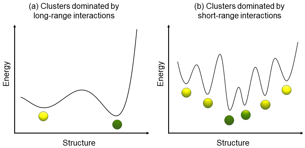
For difficult cases (large clusters, short-ranged forces, or mixed flexible/rigid systems), several independent searches with different random seeds should be run and compared. Recurrence of the same lowest-energy structure is the most practical evidence that a putative GM is reliable.
2.5. Automatic Atom Typing
Tip
The atom-typing model is described in:
Zhang, J. Atom Typing Using Graph Representation Learning: How Do Models Learn Chemistry? J. Chem. Phys. 2022, 156, 204108.
CHARMM-type force fields are much cheaper than quantum chemistry and are often the method of choice for organic molecular clusters. Their use, however, requires every atom to be assigned a CHARMM atom type that is consistent with the parameter set. In early versions of ABCluster this assignment, and the construction of the corresponding parameter files, had to be done by hand.
From ABCluster 3.1, the auxiliary program topgen performs this assignment automatically by graph representation learning. Topology adaptive graph convolutional networks (TAGCNs) were trained on more than 700 molecules with known CHARMM types. During training the networks encode chemical environment as a distribution of weights; at inference time they map an input geometry onto atom types. The user supplies coordinates; topgen returns the typing (and, where needed, bonding information for rigidmol or geom). In many cases the result is sufficiently reliable for a first global search. The types and charges should still be inspected for unusual functional groups, and physically motivated charges (for example RESP charges) may be substituted if needed.
2.6. Many-Body Energy Decomposition Analysis
Tip
The underlying electronic-structure method and the MB-EDA scheme are described in:
Zhang, J.; Tang, Z.; Zhang, X.; Zhu, H.; Zhao, R.; Lu, Y.; Gao, J. Target State Optimized Density Functional Theory for Electronic Excited and Diabatic States. J. Chem. Theory Comput. 2023, 19, 1777-1789.
Tang, Z.; Zhu, H.; Pan, Z.; Gao, J.; Zhang, J. A Many-Body Energy Decomposition Analysis (MB-EDA) Scheme based on a Target State Optimization Self-Consistent Field (TSO-SCF) Method. Phys. Chem. Chem. Phys. 2024, 26, 17549-17560.
After a GM (and its low-lying LMs) have been obtained, it is often useful to ask why the cluster is stable: whether the binding is additive, whether three-body terms stabilize or destabilize the aggregate, and which physical components dominate. Many-body energy decomposition analysis (MB-EDA), as formulated in Phys. Chem. Chem. Phys. 2024, 26, 17549, addresses these questions.
The interaction energy of an \(N\)-monomer cluster is expanded as a sum of \(n\)-body contributions:
Terms with \(n \ge 3\) are the many-body contributions. The leading many-body term is usually the three-body energy \(\Delta E^{(3)}\). Its sign has a direct chemical interpretation:
\(\Delta E^{(3)} < 0\): cooperative binding. Many-body interactions stabilize the cluster. This is common in hydrogen-bonded aggregates such as water clusters.
\(\Delta E^{(3)} > 0\): anti-cooperative binding. Many-body interactions destabilize the cluster. This is common for assemblies of charged species, such as ionic-liquid clusters.
\(\Delta E^{(3)} \approx 0\): non-cooperative binding. Many-body effects are negligible. This is typical of clusters of uncharged molecules without hydrogen bonds.
Each \(n\)-body term can be further resolved into electrostatic, exchange, polarization, charge-transfer, and dispersion contributions:
Electrostatic and exchange contributions are largely additive. Polarization and charge transfer are the principal non-additive (many-body) channels. Dispersion is additive.
MB-EDA is implemented in the quantum-chemistry program Qbics. Worked examples are given in Example: (H2O)6, Example: Li+, Na+, and Cs+ in (C6H6)6, and For Molecular Clusters: Many-Body Energy Decomposition Analysis.