Tip

All input files can be downloaded: Files.

md

This keyword controls the molecular dynamics (MD) simulation details.

Options 

Value	`NVE` Microcanonical ensemble, constant number of particles, volume, and energy
	`NVT` Canonical ensemble, constant number of particles, volume, and temperature
	`fep-NVE` Free energy perturbation calculation for microcanonical ensemble
	`fep-NVT` Free energy perturbation calculation for canonical ensemble
Default	`NVE`

Define the MD simulation type.

dt

Value	A real number
Default	`0.0005`

The time step in ps. For systems not containing hydrogen atoms, dt can be set to 0.001 ps.

num_steps

Value	An integer
Default	`10`

The number of MD steps to be run.

The total simulation time is dt``*\ ``num_steps ps.

output_freq

Value	An integer
Default	`1`

The number of steps that MD information is output. The trajectory, velocity, and gradient will be output to disk.

temp

Value	A real number
Default	`273.15`

Define the initial temperature for NVE simulation, and the targeted temperature for NVT simulation.

temp_nhc_length

Value	An integer
Default	`5`

The length of Nose-Hoover chain to control the temperature. Usually an integer larger than 2 is enough.

temp_nhc_tau

Value	A real number
Default	`0.5`

The time-constant of Nose-Hoover chain to control the temperature in ps.

vel_fn

Value	A file name
Default	None

If this is given, the initial velocities will be set from this XYZ file (in Angstrom/ps). Otherwise, velocities will be generated from Boltzmann distribution. For example:

md
  vel_fn mol-vel.xyz
end

Initial velocities will be read from mol-vel.xyz.

max_dr

Value	A real number
Default	`5`

The maximum allowed atomic displacement per step in Angstrom. If an atom mover more than max_dr in a step, Qbics will stop the MD simulation since the system may crash due to the too fast motion.

plumed_fn

Value	A file name
Default	None

If this is given, Qbics will apply enhanced sampling algorithms of PLUMED defined in this file. For PLUMED input file grammar, please refer to its PLUMED manual.

Molecular dynamics (MD) simulations are a computational method to study the time evolution of a system of interacting particles. In MD simulations, the forces between particles are calculated using a potential energy function, and the equations of motion are solved to obtain the trajectory of the particles.

In Qbics, the equations of motions are solved using the velocity-Verlet algorithm, which is a symplectic integrator, meaning that it conserves the total energy of the system over long time. The forces can be evaluated on several levels of theory, including DFT, MM, NDDO, xTB, DFT/MM, NDDO/MM, and xTB/MM.

During MD simulations, Qbics will output several files:

x-md-traj.xyz: The trajectory of the system in XYZ format.
x-md-vel.xyz: The velocity of the system in XYZ format.
x-md-grad.xyz: The gradient of the system in XYZ format. Note that force is the negative of gradient.
x-md-log.txt: The log file of the MD simulation, containing the step, time, energy components, temperature, and other information.
x-md-pressure.txt: The pressures of the MD simulation, containing the step, time, cell volume, and pressure tensor. If the system is not periodic, this file will not be generated.

If plumed_fn is given, Qbics will also output some data defined in this file.

Before doing MD, it is strongly recommended to perform a geometry optimization to obtain a stable initial configuration.

Each ensemble has its own conserved quantity.

For NVE, the total energy is conserved:

\[E = K + V\]

Here \(E\) is the total energy, \(K\) is the kinetic energy, and \(V\) is the potential energy.

For example, if you do an NVE MD simulation, you can check the total energy in file x-md-log.txt:

     #            Time                Total              Kinetic            Potential                 Temp  Cost
                    ps              Hartree              Hartree              Hartree               Kelvin  second
       0.00000         -34.44404963           0.02280104         -34.46685067         300.00000000  0.257
       0.01000         -34.44402464           0.01224859         -34.45627323         161.15837759  0.260
       0.02000         -34.44400898           0.01020550         -34.45421449         134.27682685  0.222
       0.03000         -34.44401439           0.01628312         -34.46029751         214.24190576  0.220
       0.04000         -34.44402295           0.02160569         -34.46562864         284.27246073  0.279
       0.05000         -34.44403491           0.03125266         -34.47528758         411.20057981  0.248
       0.06000         -34.44402767           0.02061378         -34.46464145         271.22164167  0.228
       0.07000         -34.44403668           0.02599444         -34.47003112         342.01656058  0.226
       0.08000         -34.44402275           0.01897475         -34.46299751         249.65643218  0.224

For NVT, the total “virtual” energy is conserved:

\[Q = K + V + \sum_{j=1}^{n_\text{NHC}} \frac{p_{\eta_j}^2}{2Q_j} + 3NkT\eta_1+kT \sum_{j=2}^{n_\text{NHC}}\eta_j\]

Here \(n_\text{NHC}\) is the Nose-Hoover chain length nhc_temp_length, \(k\) is the Boltzmann constant, \(T\) is the temperature, \(\eta_j\) and \(p_{\eta_j}\) are the thermostat variables (“position” and “momentum”), and \(Q_j\) is the thermostat mass (determined automatically by Qbics).

For example, if you do an NVT MD simulation, you can check the ConstQ in file x-md-log.txt:

     #            Time                Total              Kinetic            Potential                 Temp               ConstQ  Cost
                    ps              Hartree              Hartree              Hartree               Kelvin              Hartree  second
       0.00000         -34.44404963           0.02280104         -34.46685067         300.00000000         -34.44404963  0.000
       0.01000         -34.44404123           0.01734433         -34.46138557         228.20455596         -34.44404256  0.293
       0.02000         -34.44401539           0.01535660         -34.45937199         202.05137626         -34.44402161  0.230
       0.03000         -34.44399789           0.01914301         -34.46314090         251.87027197         -34.44401529  0.213
       0.04000         -34.44401533           0.03373382         -34.47774915         443.84591789         -34.44404524  0.303
       0.05000         -34.44399074           0.01808475         -34.46207549         237.94640025         -34.44402711  0.222
       0.06000         -34.44400165           0.03088255         -34.47488420         406.33083745         -34.44404511  0.218
       0.07000         -34.44397432           0.01350937         -34.45748370         177.74683071         -34.44402030  0.327
       0.08000         -34.44397272           0.01886731         -34.46284002         248.24278233         -34.44402353  0.222
       0.09000         -34.44398418           0.03438731         -34.47837149         452.44411562         -34.44404296  0.225

In all cases, if the conserved quantity is not conserved, it means that the simulation is unstable. You may need:

Reduce the time step;
Do a geometry optimization to obtain a stable initial configuration;
Check if the potential energy function (quantum chemistry or force field parameters) is reasonable for your system.

However, if plumed_fn is given, the conserved quantity may NOT be conserved, since the enhanced sampling algorithm may change the total energy.

Nose-Hoover Chain algorithm 

The Nose-Hoover chain (NHC) algorithm is a method to control the temperature in MD simulations. It is a generalization of the Nose-Hoover thermostat. The NHC is a series of thermostats that are connected to each other. The first thermostat controls the temperature of the system, and the subsequent thermostats control the temperature of the previous thermostat.

The length of NHC is controlled by temp_nhc_length. It should be larger than 2. If temp_nhc_length is set to 1, the system may not have a correct canonical distribution of velocities.

Input Examples 

Example: Dynamic Effects for Carbocation Reaction 

Consider the following reaction:

We want to know which group is more likely to migrate. Thus, we will do a 200 fs NVT MD simulation from the optimized structure of this carbocation to see what will happen. We will repeat the MD for 20 times using a shell script run.sh. Here we use xTB for its speed. You can also use DFT if you have enough time. The input files are shown below:

md-1.inp

mol
    C    -0.90849    0.15356    -0.48118
    C    -0.18840    -0.79035    0.24223
    C    -0.79661    -1.92884    0.73482
    C    -2.15434    -2.10431    0.51590
    C    -2.88201    -1.15101    -0.17642
    C    -2.26735    -0.01407    -0.67971
    H    -0.22972    -2.66722    1.27887
    H    -2.64692    -2.98493    0.89733
    H    -3.93966    -1.29437    -0.33076
    H    -2.84788    0.72259    -1.21038
    C    1.26411    -0.39651    0.38023
    C    -0.02903    1.30229    -0.93562
    C    1.67317    -0.22550    1.85240
    H    1.83624    -1.21169    2.27913
    H    2.60525    0.32605    1.95669
    H    0.88426    0.23363    2.45602
    C    -0.71228    2.64784    -0.65267
    H    -0.02047    3.48874    -0.70508
    H    -1.46470    2.82054    -1.41711
    H    -1.26222    2.63862    0.29289
    C    1.31204    0.95650    -0.38570
    H    2.18545    1.61818    -0.54700
    C    2.13967    -1.43173    -0.30477
    H    1.61435    -2.09539    -0.97595
    C    3.43556    -1.57292    -0.10516
    H    3.99105    -2.34108    -0.61298
    H    4.00084    -0.94936    0.56664
    C    0.38001    1.16971    -2.43593
    C    1.13470    2.39986    -2.94354
    C    -0.80675    0.90408    -3.35872
    H    1.04783    0.30446    -2.50076
    H    1.96481    2.68234    -2.30028
    H    1.54266    2.18219    -3.92659
    H    0.47031    3.25225    -3.05019
    H    -1.34333    0.00481    -3.07250
    H    -1.49736    1.74331    -3.36799
    H    -0.44263    0.76667    -4.37283
end

basis
    def2-svp
end

pseudopotential
    def2-ecp
end

scf
    charge  +1
    spin2p1  1
end

xtb
    chrg +1
end

md
    type            nvt
    dt              0.001  # 0.001 ps = 1 fs
    num_steps       200    # 0.001*200 = 0.2 ps. In real simultion, you may need > 1 ps.
    temp            300
    temp_nhc_length 5
    temp_nhc_tau    0.5
    output_freq     10     # 0.001*10 = 10 fs
end

task
    md xtb
    # md m06 # If you want to use DFT.
end

run.sh

for i in {1..20}; do
    fn=md-1-$i
    cp md-1.inp ${fn}.inp
    qbics ${fn}.inp -n 8 > ${fn}.out
done

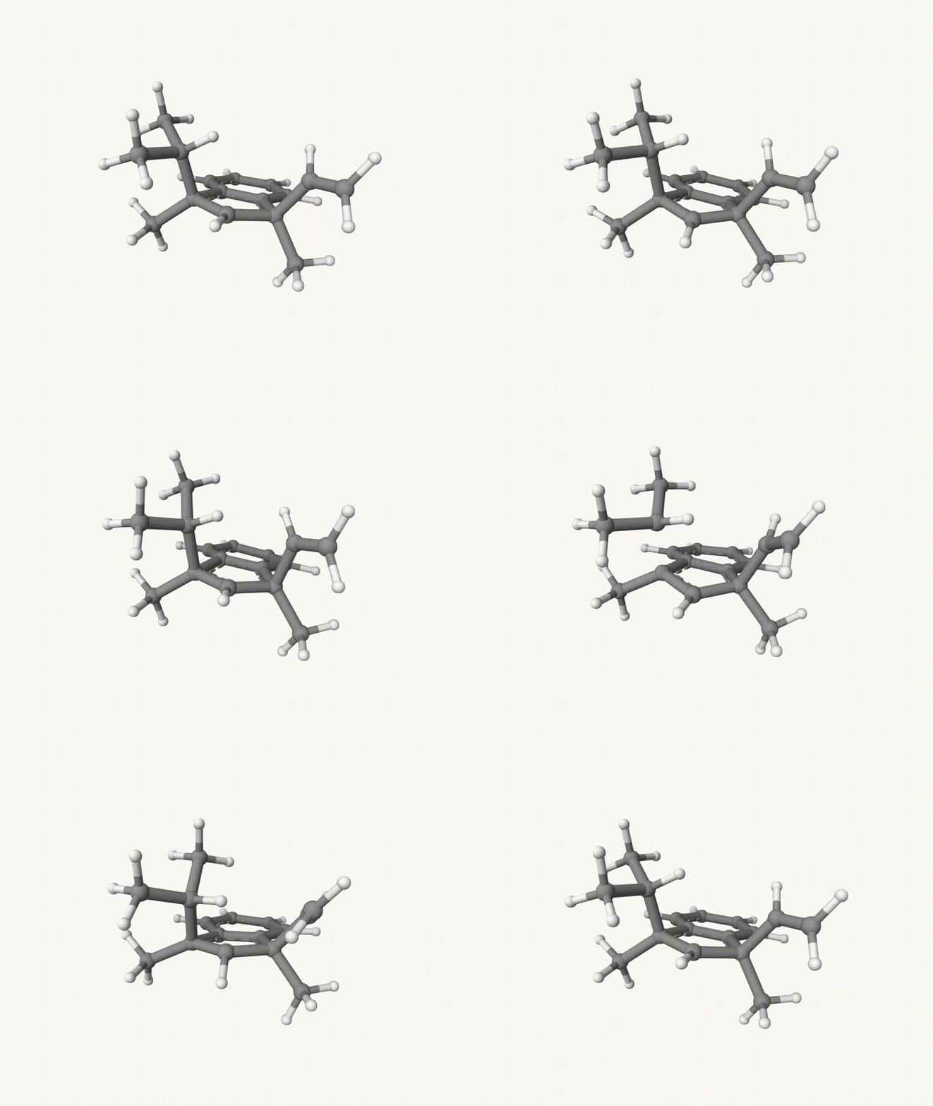
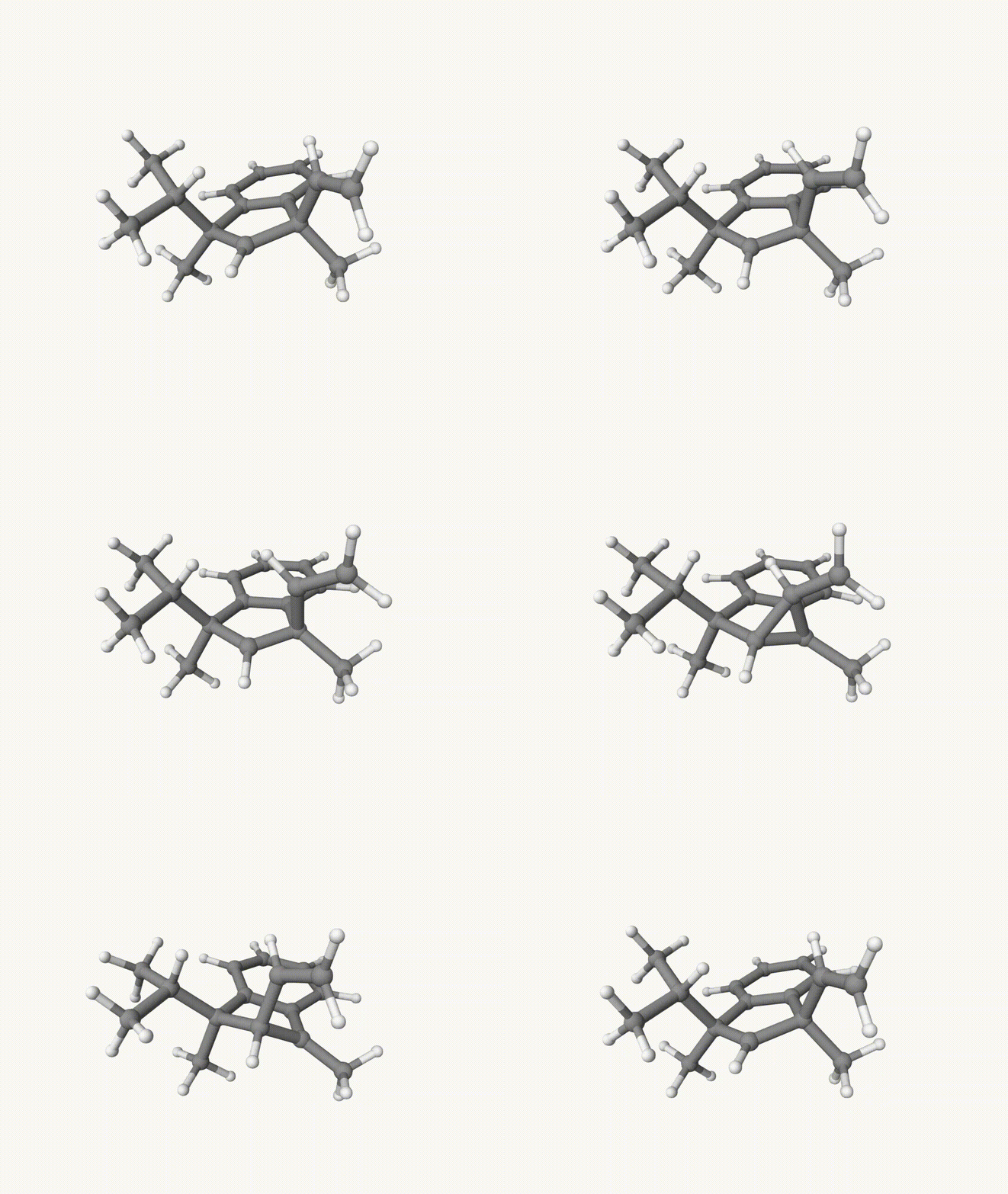
By bash run.sh, you can run 20 MD simulations. The output files will be md-1-1-md-traj.xyz, etc. We observe that both the isopropyl and vinyl group can migrate. For example:

For this test, we can calculate the migration ratio of the isopropyl group to the vinyl group. For 20 trajectories, the result is:

Isopropyl group migration	7
Vinyl group migration	7
Non-reactive	2
Other reactions	4

Of course, if the simulation time is longer, the non-reactive trajectory may become reactive. Anyway, the NVT MD result suggests that the migration ratio is about 1:1.

Why do we do dynamics? Due to the nonstatistical effect of this reaction, we cannot predict the migration ratio by a static calculation. The dynamics result is more reliable. Please refer to the paper J. Am. Chem. Soc. 2021, 143, 1088 for more details.

md

Options 

Theoretical Background 

Molecular Dynamics Simulations 

Nose-Hoover Chain algorithm 

Input Examples 

Example: Dynamic Effects for Carbocation Reaction 

md

Options

Theoretical Background

Molecular Dynamics Simulations

Nose-Hoover Chain algorithm

Input Examples

Example: Dynamic Effects for Carbocation Reaction

Options 

Theoretical Background 

Molecular Dynamics Simulations 

Nose-Hoover Chain algorithm 

Input Examples 

Example: Dynamic Effects for Carbocation Reaction 