Tip

All input files can be downloaded: Files.

Tip

Please refer to scfguess for more examples.

For a complete tutorial of TSO-DFT, please refer to:

• TSO-DFT (1): Excited States

• TSO-DFT (2): Diabatic States

scf

This option controls how to perform an SCF calculation.

Options

charge

Value	An integer
Default	0

Define the total charge of the system.

spin2p1

Value	An integer
Default	1 for even number of electrons
	2 for odd number of electrons

Define the spin multiplicity of the system, i.e., \(2S+1\), where \(S\) is the spin of the system. For example, to consider the singlet and triplet state, one should set spin2p1 to 1 and 3, respectively.

Note that spin2p1 can be either positive or negative. Both positive and negative spin2p1 represent the same spin multiplicity, but for a SCF wave function, alpha and beta orbitals will be occupied first, respectively. For example, for 11 electrons with spin2p1 being 1, there will be 6 alpha electrons and 5 beta electrons, like most quantum chemistry software does; but when spin2p1 is -1, there will be 5 alpha electrons and 6 beta electrons.

For odd number of electrons, a positive spin2p1 will first occupy alpha orbitals. If you want the beta orbitals to be occupied first, use a negative spin2p1. For example:

scf
  charge  0
  spin2p1 3
end
mol
  H 0. 0. 0.
  H 0. 0. 0.74
end

In this case, the molecule will have 2 alpha electrons and 0 beta ones. For another input:

scf
  charge  0
  spin2p1 -3
end
mol
  H 0. 0. 0.
  H 0. 0. 1.
end

The molecule will have 2 beta electrons and 0 alpha ones.

type

Value	R for restricted SCF (alpha and beta orbitals are restricted to be identical)
	U for unrestricted SCF (alpha and beta orbitals are not necessarily identical)
Default	R for singlet state
	U for other states

For singlet states, both restricted and unrestricted SCF are available. Unrestricted SCF is very useful in treating spin polarized systems. For non-singlet states, only the unrestricted one can be used.

max_it

Value	A non-negative integer
Default	128

Define the maximum number of SCF iteration.

Hint

You can set max_it to 0 to do a non-iterative calculation.

energy_cov

Value	A real number
Default	1.E-6

The energy convergence threshold for SCF calculations.

density_cov

Value	A real number
Default	1.E-8

The density matrix convergence threshold for SCF calculations.

Hint

The SCF calculation is determined to be convergent when both the energy and density convergence conditions are satisfied.

Hint

If SCF does not converge, Qbics will exit immediately. If you want Qbics to continue even an SCF calculation does not converge, please refer to output.

no_diis

Do not use direct inversion of the iterative subspace (DIIS) convergence acceleration algorithm.

no_damping

Do not use damping convergence acceleration algorithm.

damping_factor

Value	A real number
Default	0.3

The density matrix damping factor to accelerate SCF convergence.

print_MO

Print molecular orbital coefficients. Without this, only molecular orbital energies and occupancies are printed.

schwarz

Value	A real number
Default	1.E-10

Define the Schwarz screening tolerance. All two-electron integral contributions below this tolerance will be discarded to speed up calculations. A positive real number is needed.

Warning

Do not set a too large value (like 1.E-5). It may leads to wrong results.

no_scf

Value	tso Do target state optimization SCF (TSO-SCF).
	ble Do block-localized excitation SCF (BLE-SCF).
Default	None

Instead of doing ordinary SCF, do non-orthogonal SCF to treat diabatic and excited states. This is a powerful method. Some input examples can be found in scfguess. For theoretical details, please refer to:

• TSO-DFT: J. Chem. Theory Comput. 2023, 19, 1777-1789

• BLE-DFT: J. Chem. Theory Comput. 2021, 17, 240-254

Tip

For a complete tutorial of TSO-DFT, please refer to:

• TSO-DFT (1): Excited States

• TSO-DFT (2): Diabatic States.

Theoretical Background

The self-consistent field (SCF) method is the corner stone of modern electronic theory and computational chemistry. In Qbics, both Hartree-Fock and Kohn-Sham methods can be used. After calculations, energies are given in the output file, and the wave function is given in an MWFN file, which can be visualzied in Qbics-MolStar or Multiwfn.

Density Functionals

For Kohn-Sham methods, the available density functionals are listed below:

Local density approximation (LDA)

lda

Generalized gradient approximation (GGA)

pbe

blyp

bp86

olyp

pw91

pbe0

Hybrid GGA

b3lyp

o3lyp

b3pw91

x3lyp

Meta-GGA

tpss

m06l

Hybrid meta-GGA

tpssh

m06

m062x

m06hf

In modern computational chemistry, there have been a lot of experience for basis functional selection. Here, we just give a few points:

• In most cases, LDA should NOT be used.

• For organic compounds, hybrid functionals B3LYP and M06-2X are often the most reliable ones.

• For compounds containing metals, GGAs like BP86 and BLYP sometimes work better than hybrid GGAs.

Of course, the best way for basis functional selection is to do calibration for your specific system.

Also, in all modern calculations, one should use disperison corrections, like DFT-D3 in grimmedisp.

SCF Convergence

In Qbics, if an SCF does not converg, please try the following methods:

• Increase number of iterations, like mat_it 200, although in most cases this does not work;

• Set schwarz to a small value, like schwarz 1E-14;

• Use a converged wave function as the initial guess, say the same system with smaller basis sets. See scfguess for details.

Non-orthogonal SCF: TSO-DFT

XXXXXXXXXXXXXX

Non-orthogonal SCF: BLE-DFT

In QBics, the BLE (Block-Localized Excitation) method is implemented using the TSO (Two-Step Optimization) module to divide orbitals into blocks. In each block, a block-localized SCF equation is solved.

The only difference between BLE and standard TSO is in the treatment of excited-state configurations:

• BLE combines the block-SCF framework with the Δ-SCF method proposed by Peter Gill et al., rather than simply excluding certain orbitals.

• Initial Maximum Overlap Method (IMOM) is employed:

  • After the reference calculation, the excitation configuration is defined by scfguess ble.

  • The program stores the occupied orbital coefficients as \(\mathbf{C}^{\text{old}}_{\text{occ}}\).

  • These are then used to construct a new Fock matrix, which is diagonalized to obtain new coefficients \(\mathbf{C}^{\text{new}}\).

  • Instead of assigning occupations based on orbital energies, BLE uses the overlap projection between new and old occupied orbitals.

The projection is evaluated by:

\[P_q = \sum_{i\mu\nu} \left(C^{\text{old}}\right)^\dagger_{i\mu} S_{\mu\nu} C^{\text{new}}_{\nu q}\]

Orbitals with the largest projections are selected as the newly occupied orbitals.

Input Examples

Note that, in all examples below, you can change energy to opt to do geometry optimization, or md to do molecular dynamics.

Example: DFT Energy of Dieldrin

In scf-1a.inp, scf-1b.inp, and scf-1c.inp, we calculate the singlet state, triplet state, and cationic state of dieldrin. For cationic state of dieldrin, since an electron is lost, its spin is 2 so it is a doublet state. There are controled by charge and spin2p1.

scf-1a.inpscf-1b.inpscf-1c.inp

scf-1a.inp

basis
    def2-svp
end

scf
    charge  0
    spin2p1 1
end

grimmedisp
    type bj
end

mol
    Cl    1.40900    -0.54900    -0.14200
    C    2.91800    0.22200    -0.14800
    C    3.34900    1.18000    -0.99000
    Cl    2.48900    1.91800    -2.24800
    C    4.73000    1.60600    -0.53700
    Cl    5.24600    3.22500    -0.97500
    C    5.80600    0.51900    -0.74700
    C    6.83600    -0.13400    -1.70000
    C    6.40300    -1.62200    -1.82900
    C    6.19900    -1.81300    -0.26300
    C    7.62200    -1.50500    0.16600
    O    8.02000    -0.22000    0.59300
    C    8.09500    -0.42900    -0.82100
    C    5.11900    -0.73000    -0.15200
    C    4.07300    -0.11600    0.82100
    Cl    3.68500    -1.10500    2.20000
    C    4.50000    1.37200    1.05000
    Cl    5.90100    1.54700    2.17100
    Cl    3.22100    2.43400    1.80000
    H    6.52400    1.00200    -0.09500
    H    7.05500    0.38900    -2.63100
    H    7.19900    -2.27000    -2.21800
    H    5.50600    -1.77200    -2.43800
    H    5.86900    -2.82100    -0.00200
    H    8.25600    -2.36000    0.34800
    H    9.03900    -0.55400    -1.32700
    H    4.42500    -1.17200    -0.89200
end

task
    energy b3lyp
end

In the output, we can find energies:

scf-1a.outscf-1b.outscf-1c.out

scf-1a.out

Mulliken Populations
====================
     #  Symbol          Charge            Spin
----------------------------------------------
     1      Cl     -0.02667453      0.00000000
     2       C      0.00442623      0.00000000
     3       C      0.07960288      0.00000000
     4      Cl     -0.03329205      0.00000000
     5       C     -0.08518096      0.00000000
     6      Cl     -0.05476695      0.00000000
     7       C      0.16951697      0.00000000
     8       C     -0.10715159      0.00000000
     9       C      0.10427346      0.00000000
    10       C     -0.08217275      0.00000000
    11       C      0.17187228      0.00000000
    12       O     -0.26857284      0.00000000
    13       C      0.10869646      0.00000000
    14       C      0.11543761      0.00000000
    15       C      0.00080890      0.00000000
    16      Cl     -0.05286360      0.00000000
    17       C     -0.10222137      0.00000000
    18      Cl     -0.01739246      0.00000000
    19      Cl     -0.03082423      0.00000000
    20       H      0.05649853      0.00000000
    21       H     -0.00112520      0.00000000
    22       H      0.00490582      0.00000000
    23       H      0.00613081      0.00000000
    24       H     -0.00349217      0.00000000
    25       H      0.00514424      0.00000000
    26       H      0.01085963      0.00000000
    27       H      0.02755688      0.00000000
----------------------------------------------
   Sum              0.00000000      0.00000000
----------------------------------------------

Electric Multipole Moments
==========================
     #                Total           Electronic              Nuclear Unit
------------------------------------------------------------------------------------
Charge:
     0              -0.0000            -190.0000             190.0000 |e|
Dipole moment:
     X               1.5427           -4249.7734            4251.3161 Debye
     Y              -3.0998            -516.9081             513.8084 Debye
     Z              -2.9629             -61.9991              59.0362 Debye
 Total               4.5571                                           Debye
Quadrupole moment:
    XX            -131.6546          -23335.2658           23203.6113 Debye*Angstrom
    XY             -18.9204           -1824.1358            1805.2154 Debye*Angstrom
    XZ             -19.3935            -226.0675             206.6740 Debye*Angstrom
    YY            -148.1762           -2656.8691            2508.6930 Debye*Angstrom
    YZ               0.3190              50.0250             -49.7060 Debye*Angstrom
    ZZ            -149.5476           -2104.9692            1955.4216 Debye*Angstrom
------------------------------------------------------------------------------------

 ---- Self Consistent Field Energy Done ------------------

Final total energy:       -3297.20331257 Hartree

In the output files, we can find energies and propertiels like Mulliken charges and spins and electric multipole moments.

We can calculate some energies:

• Triple-singlet gap: -3297.07378259--3297.20331257 = 3.52 eV;

• Vertical electron detachment energy: -3296.89315774--3297.20331257 = 8.44 eV;

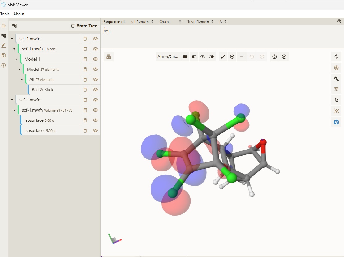
We can also visualize the molecular orbitals. Open Qbics-MolStar, and drag scf-1a.mwfn into explorer, and it will be automatically loaded. Right-click scf-1a.mwfn and select View Molecular Orbitals, 95: -0.24732 (occ=2, RHF), then the HOMO of singlet state of dieldrin is visualized:

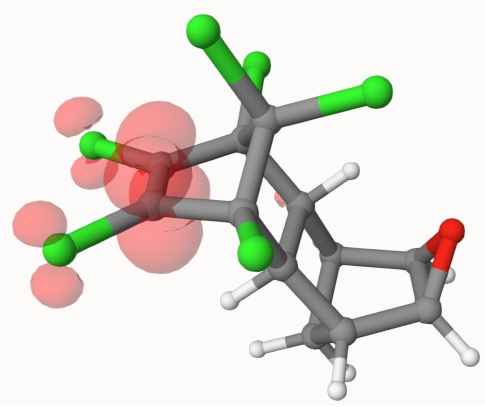
Other wavefunction proterties can be visualized. For example, dragging scf-1b.mwfn into Qbics-MolStar, and right-click scf-1b.mwfn, then click View Other Wavefunction Properties, in Format, click Electron Spin Density, you can see spin density of this system:

These works are supported by Multiwfn in the backend. Please cite Multiwfn accoring to http://sobereva.com/multiwfn if you use these data.

Example: TSO-DFT and BLE-DFT

For a detailed tutorial, please refer to:

• scfguess

• TSO-DFT (1): Excited States

• TSO-DFT (2): Diabatic States