Tip

All input files can be downloaded: Files.

Tip

For more information of this section, please refer to these keywords:

• scf

• scfguess

TSO-DFT (1): Excited States

This tutorial will lead you step by step to do target state optimization DFT (TSO-DFT) using Qbics. TSO-DFT is an originally developed method in Qbics. It is a powerful and accurate method for excited and diabatic states. In many physical processes like charge transfer, TSO-DFT can give much more reasonable results than TDDFT. Therefore, it is worth learning this method.

Hint

If you use Qbics to do TSO-DFT in you paper, please cite the following references:

• J. Chem. Theory Comput. 2023, 19, 1777

In this tutorial, we will introduce how to use TSO-DFT to study exicted states.

Example: HCHO n→π* Excitation Energy

In the first example of TSO-DFT, we will show how to calculate the n→π* excitation energy of HCHO at B3LYP/cc-pVTZ level of theory.

Hint

Accurate calculations of excited states need basis sets of high quality. We recommend cc-pVTZ or beyond for energy evaluation and cc-pVDZ or beyond for geometry optimization.

Ground State

Before studying excited states, it is always beneficial to look at the ground state first. The input for ground state is:

hcho-gs.inp

basis
    cc-pvtz
end

scf
    charge  0
    spin2p1 1
    type    R
end

mol
    O     -0.68710791      0.04339108      0.00000000
    C      0.50595906     -0.07524732      0.00000008
    H      1.09294418     -0.13258299     -0.93605972
    H      1.09294415     -0.13258317      0.93605964
end

task
    energy b3lyp
end

This is a standard SCF calculation. After calculation, we will obtain the output file hcho-gs.out and wavefunction file hcho-gs.mwfn. In hcho-gs.out, we can find these:

hcho-gs.out

SCF Structure:
 # of electrons:       16
 # of alpha electrons: 8
 # of beta electrons:  8
 2S+1:                 1
 Spin alignment:       Restricted
 Temperature:          0.00000000 Kelvin
 # of basis functions: 88

Thus, this system contains 16 electrons and 88 orbitals. We will calculate the excited states based on this information.

Excited State

The n→π* excited state is a state that an electron is excited from orbital 8 to 9. To calculate this state, one can use one of these 2 input files:

hcho-ee-1.inphcho-ee-2.inp

hcho-ee-1.inp

basis
    cc-pvtz
end

scf
    charge  0
    spin2p1 1
    type    U   # This is needed for TSO-DFT.
    no_scf  tso
end

scfguess
    type mwfn
    file hcho-gs.mwfn
    orb  16 1 1-87 : 1-7 9-88
    orb   0 1 88 : 8
end

mol
    O     -0.68710791      0.04339108      0.00000000
    C      0.50595906     -0.07524732      0.00000008
    H      1.09294418     -0.13258299     -0.93605972
    H      1.09294415     -0.13258317      0.93605964
end

task
    energy b3lyp
end

First, we claim that hcho-ee-1.inp and hcho-ee-2.inp have the same task: calculating n→π* excited state. They differ at type in scfguess...end:

• In hcho-ee-1.inp, type mwfn means that the reference state is given by a MWFN file, whose name is file hcho-gs.mwfn, that is, the ground state calculated above.

• In hcho-ee-2.inp, type tso means that the reference state is calculated automatically by Qbics. The calculated reference state will be saved to hcho-ee-2-ref.mwfn. The reference state is given by the following frag 0 1 1-4. This frag is to assign the whole molecule (atom 1-4) with charge 0 and spin multiplicity 1 as reference. See scfguess for more information.

In both hcho-ee-1.inp and hcho-ee-2.inp, the excited state is assigned by orb. In TSO-DFT, the most important concept is the partition of orbital subspace, see below:

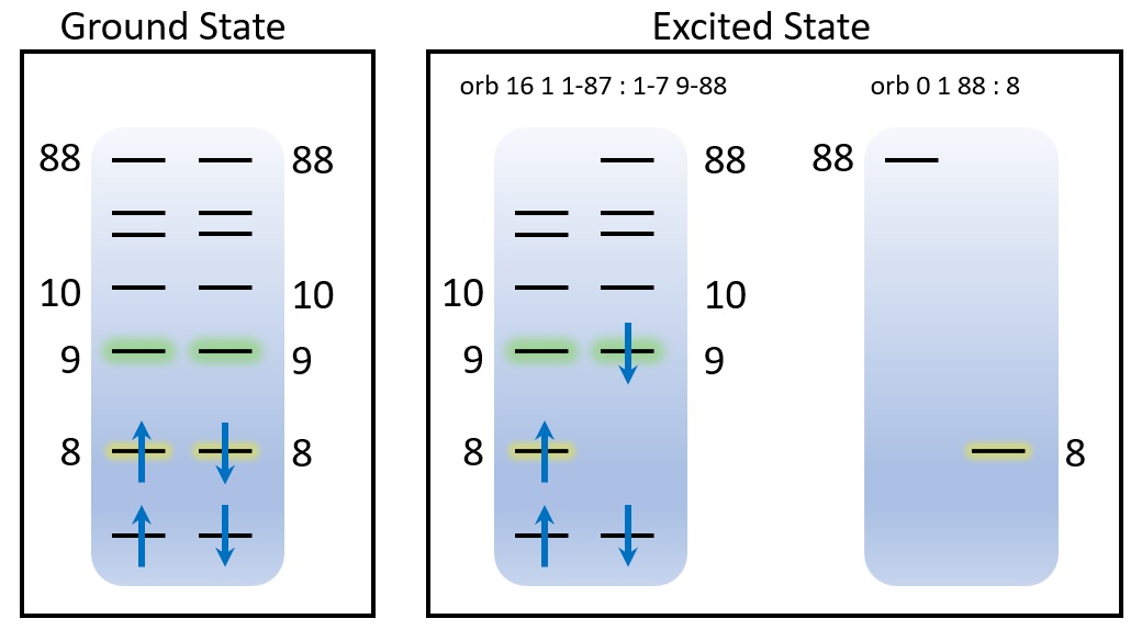
As shown by this picture, in the ground state, the alpha and beta orbitals are occupied by 8 electrons, respectively. In the n→π* excited state, i.e., the state that an electron is excited from orbital 8 to 9, we partition orbitals into 2 subspaces (2 orb):

• orb  16 1 1-87 : 1-7 9-88 The first subspace contains 16 electrons and spin multiplicity is 1. The numbers separated by : are the alpha orbital indices 1-87 and beta orbital indices 1-7 9-88, respecitively. Here, we remove beta orbital 8, so when the electrons are occupied, it will occupy 9 automatically and beta 8 is never occupied. So, an n→π* excited state is automatically constructed. Note that we also remove an alpha orbital 87, since in each orbital subspace, the number of alpha and beta orbital must be the same. Therefore, we remove the highest one.

• orb 0 1 87 : 8 The second subspace it the complementary set of the first one, so it is zero-occupied.

Now we can calculate the excited states. After calculation, we will obtain the excited state wavefunction hcho-ee-1.mwfn or hcho-ee-2.mwfn. The excited state properties can be found in hcho-ee-1.out or hcho-ee-2.out:

hcho-ee-1.out or hcho-ee-2.out

TSO Transition
==============
Reference wave function read from: hcho-ee-2-ref.mwfn
Reference energy:         -114.54951400 Hartree
Current energy:           -114.42013176 Hartree
E(Current)-E(Ref):           3.52067019 eV
Transition dipole moment (Debye):   0.00004  -0.00000  -0.00112
Oscillator strength:                0.00000
Higher order corrections:
Transition quadrupole moment (Debye*Angstrom):
 Qxx:  -0.00001; Qyy:   0.00003; Qzz:  -0.00002
 Qxy:   0.00000; Qxz:  -0.06437; Qyz:  -0.63367
Quadrupole correction to oscillator strength: 4.31049E-09
Transition angular momentum (au):   0.06258  -0.00609  -0.00032
Magnetic dipole correction to oscillator strength: 4.53975E-09

Thus, the excited energy is 3.52 eV. The oscillator strength is 0.00, suggesting that this is a dark state.

Example: HCHO n²→(π*)² Excitation Energy

Now we consider a doubly excited state, where two electons are excited from n to π*.

Hint

The popular TDDFT code in most programs are implemented with adiabatic approximation, making TDDFT unable to calculate double excitation. This is also a reason that you should use TSO-DFT: due to the theoretical flaws in TDDFT, many types of excitation, like double, core, and charge transfer excitations, cannot be studies by TDDFT, but all of them can be studied by TSO-DFT with balanced accuracy. For theoretical details, please refer to:

• J. Chem. Theory Comput. 2023, 19, 1777

To calculate this n²→(π*)² excitation, we can use one of these 2 files:

hcho-de-1.inphcho-ee-2.inp

hcho-ee-1.inp

basis
    cc-pvtz
end

scf
    charge  0
    spin2p1 1
    type    U   # This is needed for TSO-DFT.
    no_scf  tso
end

scfguess
    type mwfn
    file hcho-gs.mwfn
    orb  16 1 1-7 9-88 : 1-7 9-88
    orb   0 1 8 : 8
end

mol
    O     -0.68710791      0.04339108      0.00000000
    C      0.50595906     -0.07524732      0.00000008
    H      1.09294418     -0.13258299     -0.93605972
    H      1.09294415     -0.13258317      0.93605964
end

task
    energy b3lyp
end

These input files are very similar to the ones for n→π* excited state:

• In hcho-de-1.inp, type mwfn means that the reference state is given by a MWFN file, whose name is file hcho-gs.mwfn, that is, the ground state calculated above.

• In hcho-de-2.inp, type tso means that the reference state is calculated automatically by Qbics. The calculated reference state will be saved to hcho-de-2-ref.mwfn. The reference state is given by the following frag 0 1 1-4. This frag is to assign the whole molecule (atom 1-4) with charge 0 and spin multiplicity 1 as reference. See scfguess for more information.

The orbital partition is given below:

• orb  16 1 1-7 9-88 : 1-7 9-88 The first subspace contains 16 electrons and spin multiplicity is 1. The numbers separated by : are the alpha orbital indices 1-7 9-88 and beta orbital indices 1-7 9-88, respecitively. Here, we remove alpha/beta orbital 8, so when the electrons are occupied, they will occupy alpha/beta 9 automatically and alpha/beta 8 is never occupied. So, an n²→(π*)² doubly excited state is automatically constructed.

• orb 0 1 8 : 8 The second subspace it the complementary set of the first one, so it is zero-occupied.

Now we can calculate the excited states. After calculation, we will obtain the excited state wavefunction hcho-de-1.mwfn or hcho-de-2.mwfn. The excited state properties can be found in hcho-de-1.out or hcho-de-2.out:

hcho-de-1.out or hcho-de-2.out

TSO Transition
==============
Reference wave function read from: hcho-de-2-ref.mwfn
Reference energy:         -114.54951400 Hartree
Current energy:           -114.15687470 Hartree
E(Current)-E(Ref):          10.68425953 eV
Transition dipole moment (Debye):   0.00000   0.00000   0.00000
Oscillator strength:                0.00000
Higher order corrections:
Transition quadrupole moment (Debye*Angstrom):
 Qxx:   0.00000; Qyy:   0.00000; Qzz:   0.00000
 Qxy:   0.00000; Qxz:   0.00000; Qyz:   0.00000
Quadrupole correction to oscillator strength: 0.00000E+00
Transition angular momentum (au):   0.00000   0.00000   0.00000
Magnetic dipole correction to oscillator strength: 0.00000E+00

Thus, the excited energy is 10.68 eV.

Example: HCHO n→π* Excited State Geometry

Geometry optimization of excited states by TSO-DFT is very easy. Just remember the following 3 points:

1. Geometry optimization by TSO-DFT can only use type tso in scfguess...end;

2. Replace energy to opt;

3. Sometimes, excited state geometry have completely different symmtery from the ground state, in this case, some manually symmetry broken is needed.

The first 2 points are easy to understand. The third point will be explained by examples.

Now we want to optimize the structure of n→π* excited state of HCHO. We just need to replace energy to opt in hcho-ee-2.inp. We will call this file hcho-ee-geom-1.inp:

hcho-ee-geom-1.inp

basis
    cc-pvtz
end

scf
    charge  0
    spin2p1 1
    type    U   # This is needed for TSO-DFT.
    no_scf  tso
end

scfguess
    type tso
    frag  0 1 1-4
    orb  16 1 1-87 : 1-7 9-88
    orb   0 1 88 : 8
end

mol
    O     -0.68710791      0.04339108      0.00000000
    C      0.50595906     -0.07524732      0.00000008
    H      1.09294418     -0.13258299     -0.93605972
    H      1.09294415     -0.13258317      0.93605964
task
    opt b3lyp
end

This file will of course do the geometry optimization for excited state of HCHO. However, note that the initial geometry is a planar one, so geometry optimization will always keep this planarity. The n→π* excitation will lead to a broken of planarity of molecules, so we should give this molecule a perturbation to enable geometry optimization to treat non-planar molecules. This is given in hcho-ee-geom-2.inp:

hcho-ee-geom-2.inp

basis
    cc-pvtz
end

scf
    charge  0
    spin2p1 1
    type    U   # This is needed for TSO-DFT.
    no_scf  tso
end

scfguess
    type tso
    frag  0 1 1-4
    orb  16 1 1-87 : 1-7 9-88
    orb   0 1 88 : 8
end

mol
   O     -0.68710791      0.24339108      0.00000000 # Move O atom
   C      0.50595906     -0.27524732      0.00000008 # Move C atom
   H      1.09294418     -0.13258299     -0.93605972
   H      1.09294415     -0.13258317      0.93605964
end

task
    opt b3lyp
end

You can see that, we let C and O move out of the molecular plane by about 0.2 Angstrom.

After calculations, we can check the optimized geometry of hcho-ee-geom-1-opt.xyz and hcho-ee-geom-2-opt.xyz with Qbics-MolStar:

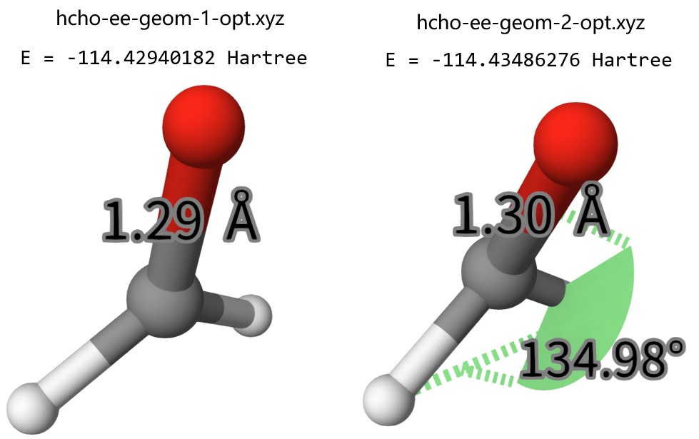
We found that, the second non-planar geometry is more stable than the planar one by 0.0054 Hartree. Interestingly, if we optimize the non-planar HCHO at ground state, it will return to the planar one. Anyway, since the potential energy surface of excited states can have completely different topology compared to the ground state one, you must take care if your excited state structure is a global minimum. Below is another example.

Example: HCCH Non-linear Excited State Geometry

HCCH is a linear molecule. Its ground state geometry can be easily determined. Now, we will determine its geometry for the HOMO→LUMO excited state, which is called S₁ state.

First, the initial structure is the ground state minimum:

hcch-1.inp

basis
    cc-pvtz
end

scf
    charge  0
    spin2p1 1
    type    U   # This is needed for TSO-DFT.
    no_scf  tso
end

scfguess
    type tso
    frag  0 1 1-4
    orb  14 1 1-87 : 1-6 8-88
    orb   0 1   88 : 7
end

mol
    H     0.0  0.0   -1.65969619
    C     0.0  0.0   -0.59806842
    C     0.0  0.0    0.59805611
    H     0.0  0.0    1.65970850
end

task
    opt b3lyp
end

However, with a linear initial guess, the local geometry optimization process can only lead to a linear molecule. Chemical intuition tells us that in the excited states, HCCH may bend. So, let’s consider 2 cases: the 2 hydrogen atoms are in cis and trans geometry. In the input file, we will simply move the 2 hydrogen atoms in the same and opposite direction, respecitvely, by a small distance:

hcch-2.inphcch-3.inp

hcch-2.inp

basis
    cc-pvtz
end

scf
    charge  0
    spin2p1 1
    type    U   # This is needed for TSO-DFT.
    no_scf  tso
end

scfguess
    type tso
    frag  0 1 1-4
    orb  14 1 1-87 : 1-6 8-88
    orb   0 1   88 : 7
end

mol
    H     0.5  0.5   -1.65969619 # Move H in the same direction
    C     0.0  0.0   -0.59806842
    C     0.0  0.0    0.59805611
    H     0.5  0.5    1.65970850 # Move H in the same direction
end

task
    opt b3lyp
end

After calculations, we collect the optimized structures in hcch-1-opt.xyz, hcch-2-opt.xyz, and hcch-3-opt.xyz, shown below:

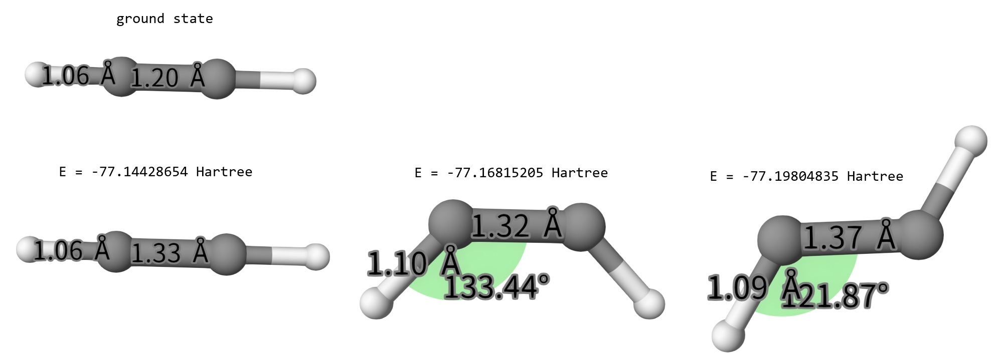
Obviously, the linear geometry is far from global optimization, being completely different from the ground state. In S₁ state, the trans isomer is the most stable one.

This example again emphasizes the compexity of excited state potential energy surfac! If you start the geometry optimization with a structure of high symmetry, you may NEVER arrive at the true minimum, so try more initial structure!