Standard Molecular Dynamics Simulations

This tutorial will lead you step by step to do standard molecular dynamics (MD) simulations using Qbics. Assume you have read Geometry Optimization, Density Functional Theory Calculations or Molecular Mechanics Calculations.

In this tutorial, we will only discuss the standard MD simulations, meaning no enhanced sampling algorithms are used. For enhanced sampling MD, please refer to Molecular Dynamics Simulations with Enhanced Sampling.

Example: NVT MD for Solvated Protein 5VBM 

Here, we will do a NVT MD simulation for the solvated protein 5VBM given in Molecular Mechanics Calculations. The input file is as follows:

5vbm-sol.inp

charmm
    # Here:
    # toppar_water_ions.str: the parameter file for water and ions.
    # par_all36m_prot.prm: the parameter file for proteins.
    # Both are obtained from website: https://mackerell.umaryland.edu/charmm_ff.shtml.
    parameters toppar_water_ions.str par_all36m_prot.prm
    topology   5vbm-sol.psf
    scaling14  1.0
    rcutoff    12.0
    rswitch    10.0
    use_PBC           # Add this line to turn on PBC.
    Lbox 70 70 70     # Define the box size.
    electrostatic pme # Use PME for electrostatics.
    PMEk   72 72 72
end

md
    type            nvt
    dt              0.001   # 0.001 ps = 1 fs
    num_steps       10000   # 10000*0.001 = 10 ps
    temp            300
    temp_nhc_length 5
    temp_nhc_tau    0.5
    output_freq     100     # 0.001*100 = 100 fs
end

mol
    5vbm-sol-opt.xyz
end

task
    opt charmm
end

Note that, in mol...end, we use the optimized structure 5vbm-sol-opt.xyz from Geometry Optimization. For biological systems, always use optimized structure as initial structure for MD simulations! Now, we will explain the options in md...end:

Line 18: The type of MD. Here we do canonical ensemble MD, which is nvt, i.e. constant number of molecules, volume, and temperature.
Line 19: The time step size of MD in ps. Usually 0.001 is a good choice. However, if there is no hydrogen atom, then 0.002 or larger can be used.
Line 20: The number of steps to do MD. Here we do 10000 steps, so the total simulation time is 10000*0.001 = 10 ps. This short time is for pedagogical purpose. In practice, one should do a much longer simulation for product analysis.
Line 21: The target temperature in Kelvin.
Line 22,23: The parameters for Nose-Hoover chain algorithm to control temperature. The parameters given here are usually OK.
Line 24: The frequency of output. Here, for every 100 steps, the coordinates, gradients, velocities, and energies are output.

After running this calculation, we have the following output:

5vbm-sol-md-traj.xyz: The trajectory.
5vbm-sol-md-vel.xyz: The velocities of all atoms for every output_freq steps.
5vbm-sol-md-grad.xyz: The gradients of all atoms for every output_freq steps.
5vbm-sol-md-log.txt: The energies for every output_freq steps.

For example:

5vbm-sol-md-log.txt

    #            Time                Total              Kinetic            Potential                 Temp               ConstQ                 Bond                Angle             Dihedral             Improper            Coulombic         LennardJones  Cost
                   ps             kcal/mol             kcal/mol             kcal/mol               Kelvin             kcal/mol             kcal/mol             kcal/mol             kcal/mol             kcal/mol             kcal/mol             kcal/mol  second
       0.00000     -134230.56945744       36085.33154757     -170315.90100501         300.00000000     -134230.56945744        6420.14428661        4495.95531110        1531.31406870          20.78944740     -209097.89905045       26313.79486581  0.129
       0.10000     -133816.54187207       16118.34524766     -149934.88711973         134.00191621     -134016.76556412        7302.41369899        5869.59861893        1666.48807052          75.45725238     -188865.46777364       24016.62295515  6.522
       0.20000     -133606.24161267       16992.08207064     -150598.32368331         141.26583857     -134065.52297681        6679.22007384        5375.41406643        1657.28109955          67.37158807     -186898.20683159       22520.59626219  6.730
       0.30000     -133300.87796459       17301.76543332     -150602.64339791         143.84043065     -134046.30803993        6874.09339659        5371.10977271        1657.72694720          75.62709833     -187077.51167460       22496.31100366  7.048
       0.40000     -132995.61549652       17629.55917628     -150625.17467280         146.56558568     -134041.03818552        6903.10388790        5646.97799910        1681.10341086
..omitted..
       9.40000     -100271.14965665       32668.17051219     -132939.32016884         271.59099649     -133856.91550183       10568.00534340        8576.31788333        1692.95053586          88.36593747     -172749.73171403       18884.77179376  7.265
       9.50000      -99959.15928496       32686.86479432     -132646.02407928         271.74641379     -133845.66058042       10659.61992276        8745.77752012        1703.07775588          96.01140798     -172661.31654362       18810.80580633  7.206
       9.60000      -99667.33935998       33043.56346211     -132710.90282209         274.71187359     -133850.81824348       10583.87601581        8824.62198457        1700.19011253          89.59345122     -173007.46226334       19098.27782584  7.214
       9.70000      -99370.72733288       32989.96543886     -132360.69277175         274.26627960     -133846.10700977       10640.12182526        8661.17837744        1693.77491115          96.10476851     -172243.89238876       18792.01968350  7.288
       9.80000      -99083.18310690       33120.13583885     -132203.31894575         275.34846780     -133847.97704020       10723.48783126        8787.10704944        1698.42095679          98.19639577     -172644.29859784       19133.76736774  7.495
       9.90000      -98790.21971731       33390.37977009     -132180.59948741         277.59517514     -133840.46539948       10862.67638260        8744.32303648        1685.93747509          97.87623972     -172406.04428515       18834.63161277  7.240
      10.00000      -98511.94567150       33524.11389736     -132036.05956887         278.70699084     -133842.52309227       10850.32141702        8657.09756469        1697.76177767          90.53706975     -172324.05730779       18992.27985877  7.197

We can see that the time, total energy, kinetic energy, potential energy, temperature and other components are output. Here, ConstQ is a conserved quantity for NVT simulation. If it strongly fluctuates during simulaiton, the MD calculation may be problematic. Also, the NVT MD is tried to keep the temperature constant at 300 K, so the temperature should not fluctuate too much. At the beginning, the temperature is around 134 K, which is not good. This means that the system has NOT been equillibrated yet. After 9 ps, the temperature is stabilized around 300 K. In practice, one should do a longer MD simulation to ensure the system is equilibrated, and then do production MD simulation.

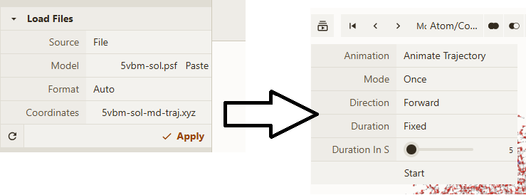
We can visualize the trajectory 5vbm-sol-md-traj.xyz in Qbics-MolStar. In Qbics, we can load topology 5vbm-sol.psf into Model and trajectory 5vbm-sol-md-traj.xyz into Coordinates, then click Apply to load the trajectory. Now click the icon in the left-up corner, and click Start. Now you can visualize the trajectory.

Now you can do various analyses on energies, trajectories, gradients, and velocities. For example, calculating diffusion coefficient, conformation change, etc.

Example: NVE MD for Bullvalene 

The MD using CHARMM force is sometimes called classic MD (CMD). Thus, the MD using quantum chemical force (like DFT, xTB) is called ab initio MD (AIMD). We can use AIMD to study dynamic effects in chemical reactions.

Below, we will do a NVE MD simulation for bullvalene. We use NVE since in this case, the system does not exchange energy with environment, thus it is an isolated system, the energy will relax within its internal degrees of freedom. We use the following input:

bullvalene-xtb.inp

xtb
    gbsa CHCl3
end

md
    type            nve
    dt              0.001   # 0.001 ps = 1 fs
    num_steps       100000  # 10000*0.001 = 10 ps
    temp            500
    output_freq     10     # 0.01*100 = 0.01 ps
end

mol
    C    -0.62880    1.05561    1.34009
    H    -0.83035    1.51659    2.30210
    C    0.13239    1.54079    0.47336
    H    0.64136    2.33325    0.99298
    C    -0.88383    -0.82066    1.33606
    H    -1.37100    -1.05330    2.29317
    C    0.79049    -0.51831    1.33499
    H    1.19125    -0.81191    2.27882
    C    0.49419    1.22452    -0.75522
    H    1.22559    1.79534    -1.30152
    C    -1.52626    -0.95189    0.16256
    H    -2.43289    -1.51994    0.39341
    C    1.56332    -0.93823    0.11905
    H    2.41452    -1.49844    0.38314
    C    -0.08122    0.08636    -1.54946
    H    -0.10037    0.16642    -2.63781
    C    -1.23434    -0.67040    -1.08946
    H    -1.91475    -1.01441    -1.86813
    C    1.16111    -0.58641    -1.09467
    H    1.84928    -0.87572    -1.88796
end

task
    md xtb
end

Here, we use xtb (with implicit solvent gbsa CHCl3) since it is much faster than DFT. Of course, you can change xtb to b3lyp to do a DFT AIMD. From md...end, we can see that we do an NVE MD for 10 ps, with a step size of 1 fs and initial temperature of 500 K.

The initial structure is a transition state. Such AIMD is sometimes called downhill dynamics. If we start the AIMD with a structure minimum (reactant), this is called uphill dynamics.

After this downhill dynamic simulaiton, we can use Qbics-MolStar to visualize the trajectory:

There are several isomerization reactions occurred. For example, during 2.00 - 3.37 ps:

which corresponds to a Cope rearrangement:

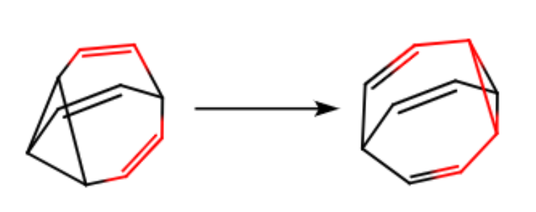
With this trajectory, you can study the reaction path or rate.

Standard Molecular Dynamics Simulations

Example: NVT MD for Solvated Protein 5VBM

Example: NVE MD for Bullvalene

Example: NVT MD for Solvated Protein 5VBM 

Example: NVE MD for Bullvalene 