Geometry Optimization

This tutorial will lead you step by step to do geometry optimization calculations using Qbics. Assume you have read Density Functional Theory Calculations or Molecular Mechanics Calculations. For optimization of transition states, please refer to Transition State Search.

Geometry optimization is to find the minimum energy structure of a molecule. It is a common task in computational chemistry and materials. As long as you can do energy calculation, simply chaning energy to opt in the input file, you can do geometry optimization.

Example: DFT for CH₃CH₂SO₃H 

For DFT, we can do geometry optimization at B3LYP-D3BJ/def2-svp level of theory for the molecule CH₃CH₂SO₃H. The input file is as follows:

ch3ch2so3h.inp

basis
    def2-svp
end

scf
    charge  0
    spin2p1 1
end

grimmedisp
    type bj
end

mol
    S    0.00000    0.00000    0.00000
    O    1.37599    0.00000    0.00000
    O    -0.71199    1.18363    0.00000
    O    -0.45996    -0.69162    -1.43483
    H    -0.82001    -0.11945    -2.10909
    C    -0.62121    -1.12008    1.07039
    H    0.14029    -1.49066    1.80382
    H    -1.47518    -0.71991    1.67461
    C    -1.14768    -2.34547    0.38391
    H    -0.34399    -2.85090    -0.10958
    H    -1.58848    -2.99835    1.10803
    H    -1.88611    -2.06128    -0.33641
end

task
    opt b3lyp
end

During optimization, Qbics will write the latest optimized structure to ch3ch2so3h-opt.xyz, and the optimization process will be written to ch3ch2so3h-opt-traj.xyz. You can visualize the optimization process using Qbics-MolStar.

After optimization, we can see the energies by this command:

$ grep "E = " ch3ch2so3h-opt-traj.xyz | cat -n
E = -703.24635624 Hartree; coordinates in Angstrom.
E = -703.25408101 Hartree; coordinates in Angstrom.
E = -703.27695102 Hartree; coordinates in Angstrom.
E = -703.28018008 Hartree; coordinates in Angstrom.
E = -703.28163730 Hartree; coordinates in Angstrom.
E = -703.28278993 Hartree; coordinates in Angstrom.
E = -703.28366187 Hartree; coordinates in Angstrom.
E = -703.28479281 Hartree; coordinates in Angstrom.
E = -703.28607847 Hartree; coordinates in Angstrom.
E = -703.28606122 Hartree; coordinates in Angstrom.
E = -703.28666766 Hartree; coordinates in Angstrom.
E = -703.28677457 Hartree; coordinates in Angstrom.
E = -703.28709275 Hartree; coordinates in Angstrom.
E = -703.28735283 Hartree; coordinates in Angstrom.
E = -703.28758537 Hartree; coordinates in Angstrom.
E = -703.28770103 Hartree; coordinates in Angstrom.
E = -703.28775039 Hartree; coordinates in Angstrom.
E = -703.28777717 Hartree; coordinates in Angstrom.
E = -703.28779907 Hartree; coordinates in Angstrom.
E = -703.28782446 Hartree; coordinates in Angstrom.
E = -703.28783816 Hartree; coordinates in Angstrom.
E = -703.28786067 Hartree; coordinates in Angstrom.
E = -703.28786999 Hartree; coordinates in Angstrom.
E = -703.28787815 Hartree; coordinates in Angstrom.
E = -703.28788727 Hartree; coordinates in Angstrom.
E = -703.28789946 Hartree; coordinates in Angstrom.
E = -703.28792996 Hartree; coordinates in Angstrom.
E = -703.28798086 Hartree; coordinates in Angstrom.
E = -703.28805214 Hartree; coordinates in Angstrom.
E = -703.28821936 Hartree; coordinates in Angstrom.
E = -703.28858252 Hartree; coordinates in Angstrom.
E = -703.28826689 Hartree; coordinates in Angstrom.
E = -703.28902797 Hartree; coordinates in Angstrom.
E = -703.28916009 Hartree; coordinates in Angstrom.
E = -703.28936878 Hartree; coordinates in Angstrom.
E = -703.28949234 Hartree; coordinates in Angstrom.
E = -703.28966812 Hartree; coordinates in Angstrom.
E = -703.28983363 Hartree; coordinates in Angstrom.
E = -703.28987269 Hartree; coordinates in Angstrom.
E = -703.29037808 Hartree; coordinates in Angstrom.
E = -703.29064316 Hartree; coordinates in Angstrom.
E = -703.29099480 Hartree; coordinates in Angstrom.
E = -703.29143705 Hartree; coordinates in Angstrom.
E = -703.29170664 Hartree; coordinates in Angstrom.
E = -703.29220829 Hartree; coordinates in Angstrom.
E = -703.29260499 Hartree; coordinates in Angstrom.
E = -703.29312866 Hartree; coordinates in Angstrom.
E = -703.29323150 Hartree; coordinates in Angstrom.
E = -703.29367916 Hartree; coordinates in Angstrom.
E = -703.29379655 Hartree; coordinates in Angstrom.
E = -703.29399614 Hartree; coordinates in Angstrom.
E = -703.29413105 Hartree; coordinates in Angstrom.
E = -703.29421491 Hartree; coordinates in Angstrom.
E = -703.29430457 Hartree; coordinates in Angstrom.
E = -703.29434373 Hartree; coordinates in Angstrom.
E = -703.29437098 Hartree; coordinates in Angstrom.
E = -703.29437738 Hartree; coordinates in Angstrom.
E = -703.29437298 Hartree; coordinates in Angstrom.
E = -703.29436155 Hartree; coordinates in Angstrom.
E = -703.29435907 Hartree; coordinates in Angstrom.
E = -703.29435586 Hartree; coordinates in Angstrom.
E = -703.29435027 Hartree; coordinates in Angstrom.
E = -703.29435261 Hartree; coordinates in Angstrom.

The energy has converged to -703.29435261 Hartree, which is the final energy of the optimized structure. It has taken 63 steps to converge.

Example: xTB Pre-optimization befor DFT Geomtry Optimization 

In the above example, the starting geometry is very bad, so it took 63 steps. Therefore, we can use xtb to do a pre-optimization before DFT optimization, which is very fast:

ch3ch2so3h-xtb.inp

basis
    def2-svp
end

scf
    charge  0
    spin2p1 1
end

grimmedisp
    type bj
end

mol
    S    0.00000    0.00000    0.00000
    O    1.37599    0.00000    0.00000
    O    -0.71199    1.18363    0.00000
    O    -0.45996    -0.69162    -1.43483
    H    -0.82001    -0.11945    -2.10909
    C    -0.62121    -1.12008    1.07039
    H    0.14029    -1.49066    1.80382
    H    -1.47518    -0.71991    1.67461
    C    -1.14768    -2.34547    0.38391
    H    -0.34399    -2.85090    -0.10958
    H    -1.58848    -2.99835    1.10803
    H    -1.88611    -2.06128    -0.33641
end

task
    opt xtb
end

This optimization only take several seconds. The final optimized structure is written to ch3ch2so3h-xtb-opt.xyz. We can use it as the starting geometry for DFT optimization:

ch3ch2so3h-dft.inp

basis
    def2-svp
end

scf
    charge  0
    spin2p1 1
end

grimmedisp
    type bj
end

mol
    ch3ch2so3h-xtb-opt.xyz
end

task
    opt xtb
end

This task takes only 17 steps to converge to -703.29434128 Hartree, which is very close to the one from direct DFT optmization, but is much faster!

Example: DFT Geomtry Optimization with Constraints 

We can apply some constraints for geometry optimization. First, let us visualize this molecule with Qbics-MolStar. Just drag ch3ch2so3h.inp into Qbics-MolStar, then right-click All, then click Add Component, then click Label in Representation, then click + Create Component, you can see clearly the atomic indices:

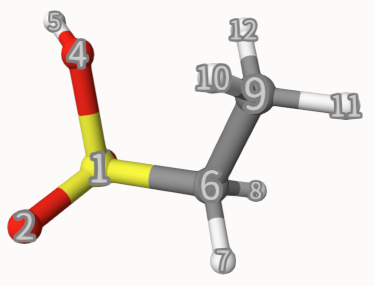
Now, we want to fix the bond 4-5 and torsion 9-6-1-4, we can use the following input:

ch3ch2so3h-cons.inp

basis
    def2-svp
end

scf
    charge  0
    spin2p1 1
end

grimmedisp
    type bj
end

opt
    fix_bond 4 5
    fix_torsion 9 6 1 4
end

mol
    S    0.00000    0.00000    0.00000
    O    1.37599    0.00000    0.00000
    O    -0.71199    1.18363    0.00000
    O    -0.45996    -0.69162    -1.43483
    H    -0.82001    -0.11945    -2.10909
    C    -0.62121    -1.12008    1.07039
    H    0.14029    -1.49066    1.80382
    H    -1.47518    -0.71991    1.67461
    C    -1.14768    -2.34547    0.38391
    H    -0.34399    -2.85090    -0.10958
    H    -1.58848    -2.99835    1.10803
    H    -1.88611    -2.06128    -0.33641
end

task
    opt b3lyp
end

This is very easy: just add constraints to opt...end. Some exmaples of constraints are:

fix_atoms 1-4 8 10-11: Fix atoms: 1 2 3 4 8 10 11;
fix_bond 4 5: Fix the bond 4-5;
fix_angle 5 7 9: Fix the angle 5-7-9;
fix_torsion 1 3 4 5: Fix the torsion 1-3-4-5.

There can be an arbitrary number of constraints. After calculation, it converge to -703.28739992 Hartree, with fixed bond length and torsion. This can also be seen with Qbics-MolStar. Drag ch3ch2so3h-cons-opt-traj.xyz into Qbics-MolStar. Then, click atom 4 and 5, and then right-click one atom, click Measure Distance to shown the bond length; for the torsion, do the similar. Then, click the icon at the left-up corner, and click Start to play the trajectory. You can see that the bond length and torsion are successfully constrained. For comparison, we also shoa a bond length that is not constrained.

Example: MM for Solvated Protein 5VBM 

For a MM system, a geometry optimization is also necessary. For the solvated protein 5VBM system given in Molecular Mechanics Calculations, we can optimize the geometry by simply changing energy to opt:

5vbm-sol.inp

charmm
    # Here:
    # toppar_water_ions.str: the parameter file for water and ions.
    # par_all36m_prot.prm: the parameter file for proteins.
    # Both are obtained from website: https://mackerell.umaryland.edu/charmm_ff.shtml.
    parameters toppar_water_ions.str par_all36m_prot.prm
    topology   5vbm-sol.psf
    scaling14  1.0
    rcutoff    12.0
    rswitch    10.0
    use_PBC           # Add this line to turn on PBC.
    Lbox 70 70 70     # Define the box size.
    electrostatic pme # Use PME for electrostatics.
    PMEk   72 72 72
end

opt
    max_step 1000
end

mol
    5vbm-sol.pdb
end

task
    opt charmm
end

However, since this system contains 40353 atoms, it will take very long to reach the strict stationary point, which is often unnecessary if it is used as an initial structure for molecular dynamic simulations. Thus, we use max_step 1000 in opt...end to limit the maximum step of optimization to 1000.

In its output 5vbm-sol.out, we can see that just in 100 steps, the enregy is optimized from the ridiculous value 11507712447667.06 kcal/mol to -146029.06 kcal/mol, which is much more reasonable. Finally, the optimized energy is -170315.90 kcal/mol.

Geometry Optimization

Example: DFT for CH3CH2SO3H

Example: xTB Pre-optimization befor DFT Geomtry Optimization

Example: DFT Geomtry Optimization with Constraints

Example: MM for Solvated Protein 5VBM

Example: DFT for CH₃CH₂SO₃H 

Example: xTB Pre-optimization befor DFT Geomtry Optimization 

Example: DFT Geomtry Optimization with Constraints 

Example: MM for Solvated Protein 5VBM 