Tip

All input files can be downloaded: Files.

qmmm

This option controls the quantum mechanics/molecular mechanics (QM/MM) calculation details.

Options 

qm_region

Value	Atom range
Default	None

Define the atoms in the QM region.

qmmm
  qm_region 1-14 16 23 45-48
end

In this input, atom 1,2,3,4,5,6,7,8,9,10,11,12,13,14,16,23,45,46,47,48 will be treated with QM methods, and others will treated with MM methods.

link

Value	`imomm` Integrated molecular-orbital molecular mechanics (IMOMM) mehtod.
	`pho` Porjected hybrid orbital (PHO) method.
Default	`imomm`

Define the method to treat of the boundary covalent bonds between QM and MM regions. In Qbics, there are two methods: imomm and pho. The imomm method will add a hydrogen atom to saturate the boundary valency; the pho method will not add any hydrogen atom, but will use a special set of projected hybrid orbital to treat the boundary covalent bonds. Both methods are implmented in a black-box manner, and users do not need to worry about the details of the methods. Their details can be found in the references below.

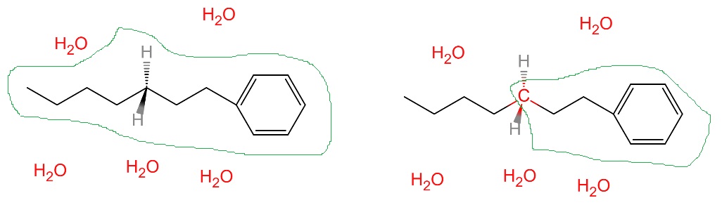
In Qbics, “covalent bonds” are defined in the PSF file (given by topology in charmm). In the QM region, all bonds are possible to break and form, while in the MM region, covalent bonds defined in the PSF file NEVER break and form. The boundary covalent bonds between QM and MM regions are NOT allowed to break. In the figure below, the QM region is defined by the green circle. For the left case, since no covalent bonds are defined between QM and MM regions, the link option is ignored (no matter what value given). For the right case, there are 3 covalent bond between QM and MM regions (red bonds), and the link option is used to treat these bonds.

In Qbics, only sp³ carbon can be used at the boundary (It must be included in the QM region).

Both methods can treat the boundary covalent bonds. The pho method is more accurate for ground states; but imomm method can be combined with TSO- or BLE-SCF (see scf) to calculate the excited and diabatic states.

Theoretical Background 

Quantum Mechanics / Molecular Mechanics (QM/MM) is a multiscale computational strategy that combines the accuracy of quantum-mechanical (QM) methods for a chemically active region with the speed of molecular-mechanical (MM) force fields for the surrounding environment. In Qbics, the QM region can be treated with DFT, xTB, or NDDO methods, while the MM region is typically described by CHARMM or AMBER force fields. This approach allows for efficienzt simulations of large chemical systems.

To do QM/MM simulations, first one have to prepare force field parameters and topology for the whole system, then use qm_region to define the QM region. If there ARE covalent bonds between atoms in QM and MM region, the boundary atoms must be sp³ carbon (i.e., carbon atom linking to 4 atoms). Other atoms are NOT supported to be boundary. This is a reasonable restriction since in these cases the molecular orbitals can be significantly delocalized over QM and MM region, those bonds should not be cut. Based on link option, Qbics will call the corresponding method to treat boundary atoms.

There are two methods for link: imomm and pho. The IMOMM method adds a hydrogen atom to saturate the boundary valency, while the PHO method uses a special set of projected hybrid orbitals to treat these bonds without adding hydrogen atoms. Both methods are implemented in a black-box manner, allowing users to focus on their calculations without needing to understand the underlying details. The main points are:

IMOMM: will add additional hydrogen atoms. Can be used for both ground and excited states.*
PHO: will NOT add any additional atoms. Can only be used for ground states.

Input Examples 

Example: Solvated Organic Anion 

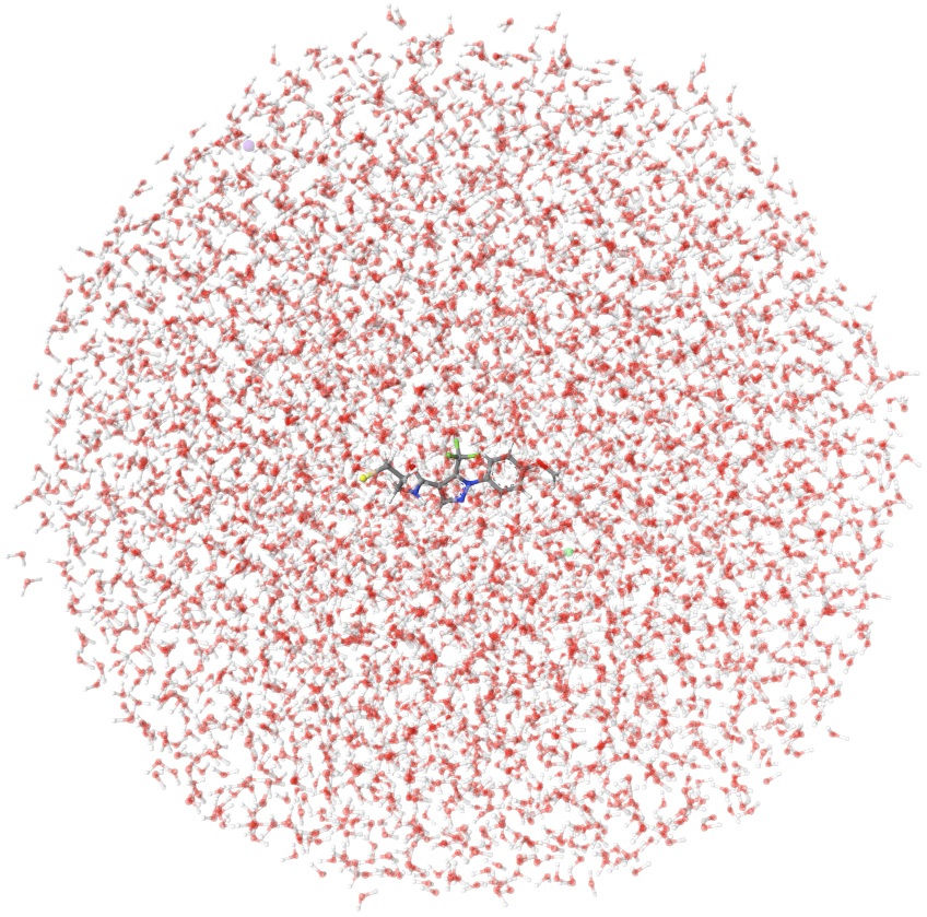
In this example, we will do a QM/MM calculation for a water microdroplet of an organic anion. The input is given below:

qmmm-1a.inp

charmm
    parameters toppar_water_ions.str 92v-1-naive.prm
    topology   92v-solvate.psf
    scaling14  1.0
    rcutoff    12.0
    rswitch    100.0 # rswitch>rcutoff means no cutoff is applied.
end

xtb
    chrg -1 # The charge in QM region!
    uhf   0 # The number of unpaired electrons in QM region!
end

qmmm
    qm_region 1-39
end

opt
    max_step 2000
end

mol
    92v-solvate.pdb
end

task
    opt xtb/charmm
end

In qmmmm-1a.inp, we have given the charmm and xtb blocks to define the force field parameters and the QM method. The mol block is used to load the cooridnates; The topology is defined in the PSF file (topology in charmm); the parameters are defined in parameters in charmm. The task block is used to run the optimization with QM/MM method. Note that this is a gas phase optimization, so no cutoff is applied (rswitch is set to be larger than rcutoff).

Another important point is that in xtb, the charge and number of unpaired electrons are defined only for in the QM region!

After optimization, the structure is stored in qmmm-1a-opt.xyz, shown below:

We can use it as the structure to do a B3LYP-D3BJ/def2-svp single point energy:

qmmm-1b.inp

charmm
    parameters toppar_water_ions.str 92v-1-naive.prm
    topology   92v-solvate.psf
    scaling14  1.0
    rcutoff    12.0
    rswitch    100.0 # rswitch>rcutoff means no cutoff is applied.
end

xtb
    chrg -1 # The charge in QM region!
    uhf   0 # The number of unpaired electrons in QM region!
end

basis
    def2-svp
end

scf
    charge  -1 # The charge in QM region!
    spin2p1  1 # The spin multiplicity in QM region!
end

grimmedisp
    type bj
end

qmmm
    qm_region 1-39
end

mol
    qmmm-1a-opt.xyz
end

task
    energy b3lyp/charmm
end

At the end of qmmm-1b.out, you can find this:

qmmm-1b.out

Total QM/MM energy
==================
Polarized QM energy:      -1608.98518142 Hartree
Whole system MM energy:     -90.52845586 Hartree
QM/MM energy correction:     16.29439183 Hartree
------------------------------------------------
QM/MM energy:             -1683.21924545 Hartree

Final total energy:       -1683.21924545 Hartree

QM/MM energy is the total energy.

In all above cases, you can change energy or opt to md to do a QM/MM MD simulation.

Example: Residues in Solvated Protein 

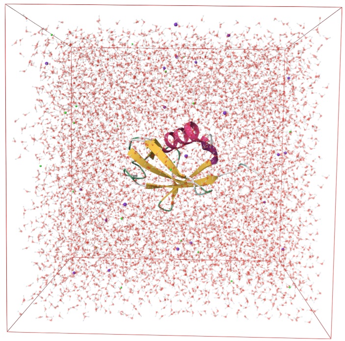
In this example, we will show the QM/MM energy calculation of two interacting residues in a protein. Assume we have already prepared a solvated protein, shown below:

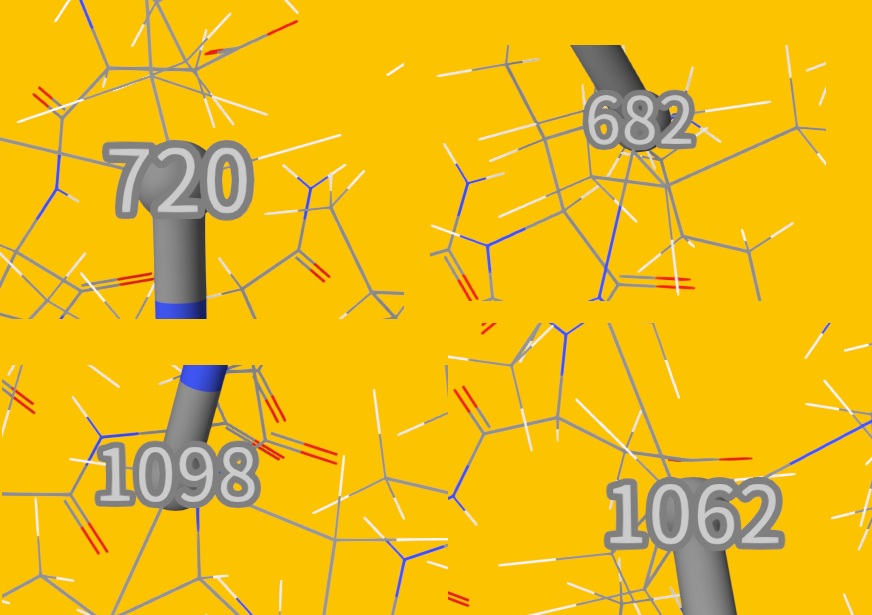
We will choose two residues on a beta-sheet region, i.e. ILE44 and HSD68, which are far away from each other on sequence but are quite close in 3D space. We also include some of their neighboring atoms. The atom indices are shown below:

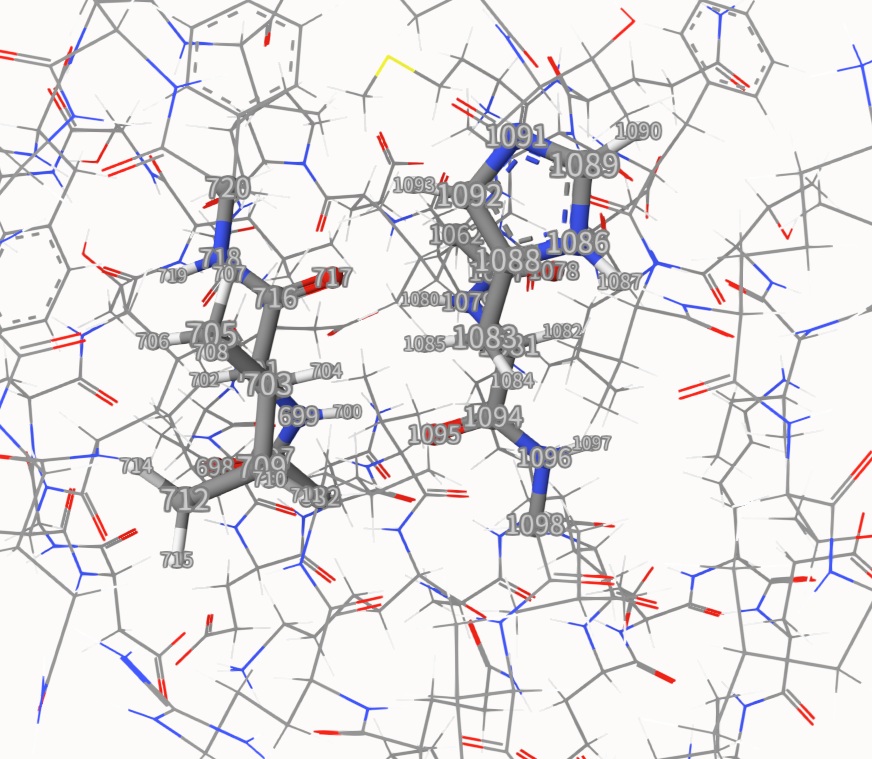
The QM region is cut at 4 sp³ carbon atoms, also shown below. All boundary carbon atoms link to 3 MM atoms:

Thus, the input file is:

qmmm-2.inp

charmm
    parameters toppar_water_ions.str par_all36m_prot.prm
    topology   sys.psf
    scaling14  1.0
    rcutoff    12.0
    rswitch    10.0
    use_PBC         # Add this line to turn on PBC.
    Lbox 64 64 64   # Define the box size.
    electrostatic cutoff # Use cutoff or QM/MM.
end

basis
    def2-svp
end

scf
    charge  0
    spin2p1 1
end

qmmm
    qm_region 682 697-720 1062 1077-1098
    link imomm # or change to: pho
end

mol
    sys.xyz
end

task
    energy b3lyp/charmm
end

The above input should be self-explanatory, if you have already known how to use Qbics to do QM and MM calculations. The only point is that currently, if the periodic boundary condition (PBC) is turned on, it is recommended to use cutoff instead of pme for QM/MM calculations.

After calculation, you can find the following lines:

qmmm-2.out

Link atoms algorithm: IMOMM
Boundary:
 QM atom 682: A hydrogen is capped at (2.484, -2.583, 3.898) Angstrom.
  MM atom 680 has 2 bonded MM atoms: 678 681
  MM atom 683: No MM atoms bond to it.
  MM atom 684 has 3 bonded MM atoms: 685 686 687
 QM atom 697: No MM atoms bond to it.
...omitted...
 QM atom 720: A hydrogen is capped at (-2.116, -2.240, 7.935) Angstrom.
  MM atom 721: No MM atoms bond to it.
  MM atom 722 has 3 bonded MM atoms: 723 724 725
  MM atom 736 has 2 bonded MM atoms: 737 738
 QM atom 1062: A hydrogen is capped at (-1.980, 2.584, 5.141) Angstrom.
  MM atom 1060 has 2 bonded MM atoms: 1058 1061
  MM atom 1063: No MM atoms bond to it.
  MM atom 1064 has 3 bonded MM atoms: 1065 1066 1067
...omitted...
Total QM/MM energy
==================
Polarized QM energy:      -1200.63363221 Hartree
Whole system MM energy:    -178.02621763 Hartree
QM/MM energy correction:     23.67074974 Hartree
------------------------------------------------
QM/MM energy:             -1354.98910010 Hartree

Final total energy:       -1354.98910010 Hartree

Lines 1-16 show how Qbics is treating the boundary atoms, the remaining lines are the QM/MM energies.

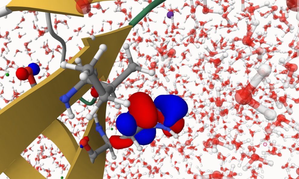
You can also visualize electronic structures with Qbics-MolStar. Load topology sys.psf in Model and coordinates sys.xyz in Coordinates, click Apply to load the solvated protein. Then, drag qmmm-2.mwfn into Qbics-MolStar to loead wavefunction. Then, right-click qmm-2.mwfn, click View Molecular Orbitals, click 91: -0.36206 (occ=2,RHF), then the HOMO of this system is shown below. The QM region is rendered using ball-and-stick representation.

You can also visualize other properties with Qbics-MolStar.

qmmm

Options

Theoretical Background

Input Examples

Example: Solvated Organic Anion

Example: Residues in Solvated Protein