Tip
All input files can be downloaded: Files.
wfn
This keyword controls the details of wave function analysis.
Options
- file
Value
File name
Default
None
The file name of the wave function to be analyzed (in MWFN format).
- loc_max_it
Value
An integer
Default
500The maximum number of steps for orbital localization.
- loc_cov
Value
A real number
Default
1.E-6The convergence threshold for orbital localization.
- print_MO_details
When this keyword is presented, much more information will be output for orbital component analysis.
Theoretical Background
In Qbics, quantum chemical calculations will produce a wavefunction and store it in a MWFN file. This is a format that contains all the information about the wavefunction, including the molecular coordinates and orbitals. Qbics can read this file and perform some simple wavefunction analysis:
Orbital localization: The wavefunction can be localized on atoms. Qbics uses Boys algorithm.
Orbital component analysis: The wavefunction can be analyzed in terms of the atomic orbitals.
For more kinds of wavefunction analysis, one can use Qbics-MolStar, which uses Multiwfn as the backend. Please refer to http://sobereva.com/multiwfn/ for more details and correct citation.
Input Examples
Example: Wavefunction Analysis for CH2O
Now we perform a wavefunction analysis for CH2O. The input file is as follows:
wfn-1.inp1basis 2 def2-tzvp 3end 4 5wfn 6 file wfn-1.mwfn # The file name. 7 print_MO_details # Print more information. 8end 9 10mol 11 O -0.00000001 -0.00000000 1.44310862 12 C -0.00000001 -0.00000000 0.24425258 13 H 0.00000004 0.93861213 -0.34368060 14 H -0.00000002 -0.93861212 -0.34368059 15end 16 17task 18 energy b3lyp # Do an energy calculation and generate wavefunction file: wfn-1.mwfn 19 wfn # Do analysis. 20end
AFter calculation, there will be 2 MWFN files
wfn-1.mwfn: Stores the original canonical molecular orbitals;wfn-1-loc.mwfn: Stores the localized molecular orbitals.
The output file also contains atomic orbital components:
wfn-1.out1Molecular orbitals: 2 # Occ O1 C2 H3 H4 3 total S P D F total S P D F total S P D F total S P D F 4 1 2.000 0.9997 0.9989 0.0008 0.0000 0.0000 0.0003 0.0001 0.0001 0.0000 0.0000 0.0000 0.0000 0.0000 0.0000 0.0000 0.0000 0.0000 0.0000 0.0000 0.0000 5 2 2.000 0.0009 0.0004 0.0005 0.0000 0.0000 0.9987 0.9986 0.0001 0.0000 0.0000 0.0002 0.0002 0.0000 0.0000 0.0000 0.0002 0.0002 0.0000 0.0000 0.0000 6 3 2.000 0.9743 0.7996 0.1746 0.0001 0.0000 0.0254 0.0195 0.0058 0.0001 0.0000 0.0001 0.0001 0.0000 0.0000 0.0000 0.0001 0.0001 0.0000 0.0000 0.0000 7 4 2.000 0.0168 0.0028 0.0138 0.0002 0.0000 0.5906 0.2875 0.3020 0.0011 0.0000 0.3588 0.3571 0.0017 0.0000 0.0000 0.0338 0.0337 0.0001 0.0000 0.0000 8 5 2.000 0.0168 0.0028 0.0138 0.0002 0.0000 0.5906 0.2875 0.3020 0.0011 0.0000 0.0338 0.0337 0.0001 0.0000 0.0000 0.3588 0.3571 0.0017 0.0000 0.0000 9 6 2.000 0.5884 0.1161 0.4708 0.0014 0.0000 0.4027 0.1686 0.2318 0.0020 0.0003 0.0044 0.0044 0.0001 0.0000 0.0000 0.0044 0.0044 0.0001 0.0000 0.0000 10 7 2.000 0.6737 0.0000 0.6716 0.0021 0.0001 0.3259 0.0000 0.3233 0.0024 0.0002 0.0002 0.0000 0.0002 0.0000 0.0000 0.0002 0.0000 0.0002 0.0000 0.0000 11 8 2.000 0.8530 0.0000 0.8519 0.0010 0.0001 0.0327 0.0000 0.0282 0.0044 0.0001 0.0572 0.0571 0.0000 0.0000 0.0000 0.0572 0.0571 0.0000 0.0000 0.0000 12 9 0.000 0.4390 0.0000 0.3370 0.0959 0.0061 0.5510 0.0000 0.3801 0.1369 0.0340 0.0050 0.0000 0.0050 0.0000 0.0000 0.0050 0.0000 0.0050 0.0000 0.0000 13 10 0.000 0.0122 0.0007 0.0114 0.0001 0.0000 0.4747 0.3168 0.1506 0.0060 0.0013 0.5084 0.4970 0.0113 0.0000 0.0000 0.0047 0.0046 0.0001 0.0000 0.0000 14 11 0.000 0.4033 0.3157 0.0827 0.0049 0.0001 0.5946 0.3464 0.2090 0.0375 0.0018 0.0010 0.0010 0.0000 0.0000 0.0000 0.0010 0.0010 0.0000 0.0000 0.0000 15 12 0.000 0.0122 0.0007 0.0114 0.0001 0.0000 0.4747 0.3168 0.1506 0.0060 0.0013 0.0047 0.0046 0.0001 0.0000 0.0000 0.5084 0.4970 0.0113 0.0000 0.0000 16 13 0.000 0.0222 0.0053 0.0167 0.0001 0.0000 0.7300 0.5137 0.2093 0.0054 0.0016 0.2469 0.2432 0.0037 0.0000 0.0000 0.0010 0.0009 0.0001 0.0000 0.0000 17 14 0.000 0.3324 0.0000 0.1867 0.1329 0.0128 0.6647 0.0000 0.1752 0.3333 0.1562 0.0015 0.0000 0.0015 0.0000 0.0000 0.0015 0.0000 0.0015 0.0000 0.0000 18 15 0.000 0.0222 0.0053 0.0167 0.0001 0.0000 0.7300 0.5137 0.2093 0.0054 0.0016 0.0010 0.0009 0.0001 0.0000 0.0000 0.2469 0.2432 0.0037 0.0000 0.0000 19... 20Quantitative atomic contributions for molecular orbitals: 21 22Molecular orbitals: 23 1, occ = 2.000, over 1 centers: O1(99.97%), ==> S(99.91%) + P(0.09%) + D(0.00%) + F(0.00%) 24 2, occ = 2.000, over 1 centers: C2(99.87%), ==> S(99.93%) + P(0.07%) + D(0.00%) + F(0.00%) 25 3, occ = 2.000, over 1 centers: O1(97.43%), ==> S(81.93%) + P(18.04%) + D(0.02%) + F(0.00%) 26 4, occ = 2.000, over 2 centers: C2(59.06%), H3(35.88%), ==> S(68.11%) + P(31.75%) + D(0.13%) + F(0.00%) 27 5, occ = 2.000, over 2 centers: C2(59.06%), H4(35.88%), ==> S(68.11%) + P(31.75%) + D(0.13%) + F(0.00%) 28 6, occ = 2.000, over 2 centers: O1(58.84%), C2(40.27%), ==> S(29.35%) + P(70.27%) + D(0.34%) + F(0.04%) 29 7, occ = 2.000, over 2 centers: O1(67.37%), C2(32.59%), ==> S(0.00%) + P(99.53%) + D(0.45%) + F(0.03%) 30 8, occ = 2.000, over 1 centers: O1(85.30%), ==> S(11.42%) + P(88.03%) + D(0.53%) + F(0.02%) 31 9, occ = 0.000, over 2 centers: O1(43.90%), C2(55.10%), ==> S(0.00%) + P(72.70%) + D(23.28%) + F(4.02%) 32 10, occ = 0.000, over 2 centers: C2(47.47%), H3(50.84%), ==> S(81.91%) + P(17.35%) + D(0.60%) + F(0.14%) 33 11, occ = 0.000, over 2 centers: O1(40.33%), C2(59.46%), ==> S(66.41%) + P(29.17%) + D(4.24%) + F(0.18%) 34 12, occ = 0.000, over 2 centers: C2(47.47%), H4(50.84%), ==> S(81.91%) + P(17.35%) + D(0.60%) + F(0.14%) 35 13, occ = 0.000, over 2 centers: C2(73.00%), H3(24.69%), ==> S(76.31%) + P(22.98%) + D(0.55%) + F(0.16%)
For example, Line 11 and 30 shows that the molecular orbital 8 has an occupation number of 2.000 and is localized on the oxygen atom (O1) with a contribution of 85.30%. The orbital is mainly composed of the s orbital (11.42%) and p orbital (88.03%). This is actually an electron lone pair orbital.
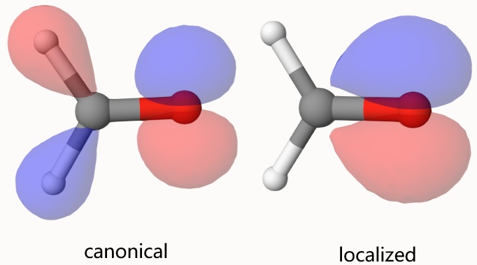
Using Qbics-MolStar to open wfn-1.mwfn and wfn-1-loc.mwfn, we can visualize the canonical and localized orbitals. For example, right-click wfn-1.mwfn and select View Molecular Orbitals, then select the orbital you want to visualize. Below is an example. Obviously, the canonical orbital is delocalized over the molecule while the localized one is only localized over a bond.